Given:
    data – a set of observed data points
    model – a model that can be fitted to data points
    n – the minimum number of data values required to fit the model
    k – the maximum number of iterations allowed in the algorithm
    t – a threshold value for determining when a data point fits a model
    d – the number of close data values required to assert that a model fits well to data

Return:
    bestfit – model parameters which best fit the data (or nul if no good model is found)

iterations = 0
bestfit = nul
besterr = something really large
while iterations < k {
    maybeinliers = n randomly selected values from data
    maybemodel = model parameters fitted to maybeinliers
    alsoinliers = empty set
    for every point in data not in maybeinliers {
        if point fits maybemodel with an error smaller than t
             add point to alsoinliers
    }
    if the number of elements in alsoinliers is > d {
        % this implies that we may have found a good model
        % now test how good it is
        bettermodel = model parameters fitted to all points in maybeinliers and alsoinliers
        thiserr = a measure of how well model fits these points
        if thiserr < besterr {
            bestfit = bettermodel
            besterr = thiserr
        }
    }
    increment iterations
}
return bestfit
defransac(data, model, n, k, t, d): ''' data – a set of observed data points model – a model that can be fitted to data points n – the minimum number of data values required to fit the model k – the maximum number of iterations allowed in the algorithm t – a threshold value for determining when a data point fits a model d – the number of close data values required to assert that a model fits well to data Return: bestfit – model parameters which best fit the data (or nul if no good model is found) ''' train_data_x = [[data[0][i]] for i in range(len(data[0]))] train_data_y = data[1] iterations = 0 bestfit = 0 besterr = 10000 while iterations < k: indexes = [rnd.randrange(0, len(data[0])) for i in range(n)] maybeinliners_x = [train_data_x[i] for i in indexes] maybeinliners_y = [train_data_y[i] for i in indexes] maybemodel = model.fit(maybeinliners_x, maybeinliners_y) alsoinliers = set() predict = maybemodel.predict(train_data_x) for i in range(len(train_data_x)): points_x = train_data_x[i] if points_x notin maybeinliners_x: data_loss = loss(train_data_y[i], predict[i]) if data_loss < t: alsoinliers.add((points_x[0], train_data_y[i])) if len(alsoinliers) > d: # this implies that we may have found a good model # now test how good it is inliers_x = [[point[0]] for point in alsoinliers] inliers_y = [point[1] for point in alsoinliers] inliers_x.extend(maybeinliners_x) inliers_y.extend(maybeinliners_y) bettermodel = model.fit(inliers_x, inliers_y) predict = maybemodel.predict(inliers_x) thiserr = np.sqrt(np.average( (inliers_y - predict) ** 2)) if thiserr < besterr: besterr = thiserr bestfit = bettermodel iterations = iterations + 1 return bestfit
DEMO
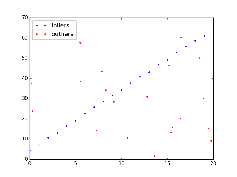
生成了一部分可以用直线拟合的数据和一些随机噪声,比例为 \(1:1\) ,如下图所示:
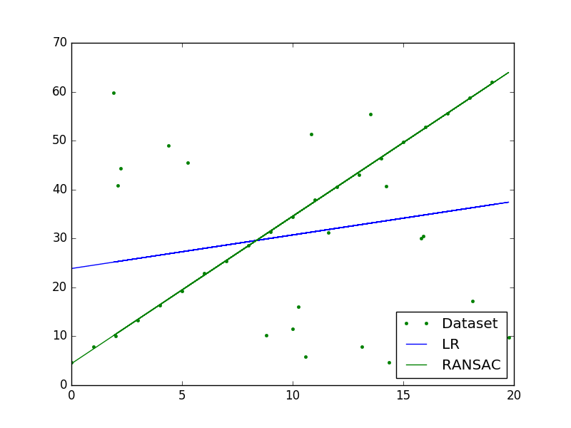
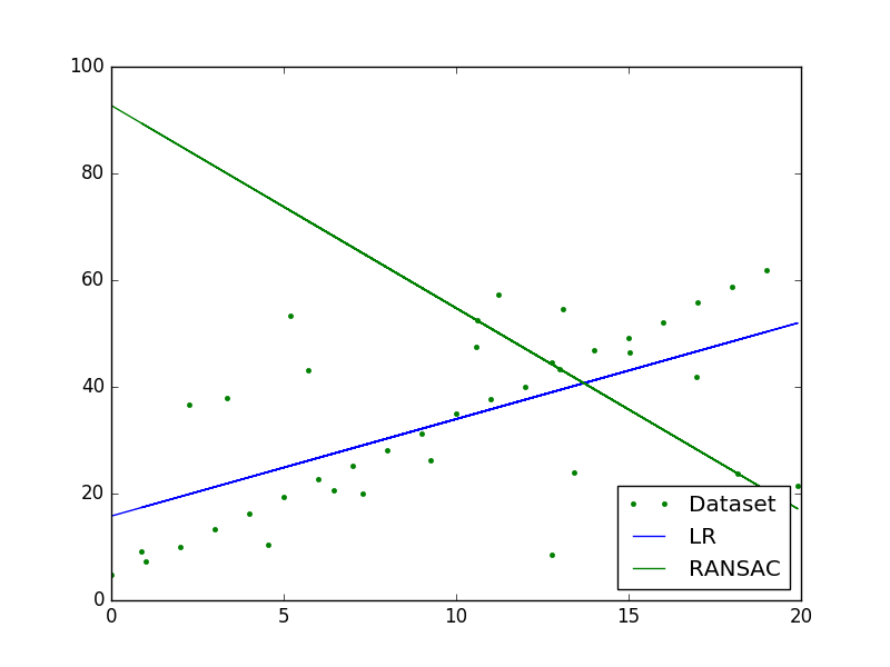
用线性回归直接拟合和RANSAC算法的结果:
Parameters
RANSAC算法中有几个超参数需要调试:
t, d : 这两个参数需要根据应用和数据集来调节
k(最大迭代次数):可以从理论上确定。
定义 \(p\) 是RANSAC算法在某次迭代采样时只采样到正常样本的概率。如果这真的发生了,那么这次迭代将训练出一个很好的模型,所以 \(p\) 也代表了RANSAC算法得出一个好结果的概率。再定义 \(w\) 为每次采样时,采到一个正常点的概率,即 \(w\) = number of inliers in data / number of points in data。假设一次采样选取 \(n\) 的样本,那么这次采样选择的样本全部都是正常样本的概率为 \(w^n\)(假设为放回采样),至少选择一个异常样本的概率就为 \(1-w^n\)。总共迭代 \(k\) 次,那么这 \(k\) 次采样都至少有一个异常样本的概率为:\((1-w^n)^k\),应该等于 \(1-p\),即 \[
1-p=(1-w^n)^k
\] 两边同时取对数得: \[
k = \frac{\log(1-p)}{\log(1-w^n)}
\] 实际上我们是不放回采样,所以还要在上面的基础上加上 \(k\) 的标准差。\(k\) 的标准差定义为: \[
SD(k) = \frac{\sqrt{1-w^n}}{w^n}
\]