Table of Contents
- The Elasticity of Demand
- The Price Elasticity of Demand and Its Determinants
- Computing the Price Elasticity of Demand
- The Midpoint Method: A Better Way To Calculate Percentage Changes and Elasticities
- The Variety of Demand Curves
- Total Revenue and The Price Elasticity of Demand
- Elasticity and Total Revenue Along A Linear Demand Curve
- Other Demand Elasticities
- The Elasticity Of Supply
- Three Applications Of Supply, Demand, And Elasticity
- The Distributional Effects of Tax
The Elasticity of Demand
To measure how much consumers respond to changes in economic variables, economists use the concept of elasticity. Elasticity is a measure of the responsiveness of quantity demanded or quantity supplied to one of its determinants.
The Price Elasticity of Demand and Its Determinants
The price elasticity of demand measures how much the quantity demanded responds to a change in price. Demand for a good is said to be elastic if the quantity demanded responds substantially to changes in the price. Demand is said to be inelastic if the quantity demanded responds only slightly to changes in the price.
Based on experience, however, we can state some general rules about what determines the price elasticity of demand.
- Availablity of Close Substitutes
- Necessities versus Luxuries
- Definition of the Market
- Time Horizon
Computing the Price Elasticity of Demand
Price elasticity of demand = Percentage change in quantity demanded / Percentage change in price
For example, suppose that a 10 percent increase in the price of an ice-cream cone causes the amount of ie cream you buy to fall by 20 percent. We calculate your elasticity of demand as
Price elasticity of demand = 20 percent / 10 percent = 2.
In this example, the elasticity is 2, reflecting that the change in the quantity demanded is proportionately twice as large as the change in the price. A larger price elasticity implies a greater responsiveness of quantity demanded to price.
The Midpoint Method: A Better Way To Calculate Percentage Changes and Elasticities
The elasticity from point A to point B seems different from the elasticity from point B to point A. This difference arises because the percentage changes are calculated from a different base.
One way to avoid this problem is to use the midpoint method for calculating elasticities. The midpoint method computes a percentage change by dividing the midpoint of the initial and final levels. The following formula expresses the midpoint method for calculating the price elasticity of demand between two points, denoted (Q1, P1) and (Q2, P2):

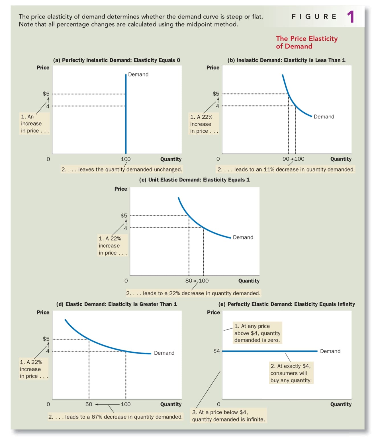
The Variety of Demand Curves
Demand is considered elastic when the elasticity is greater than 1. Demand is considered inelastic when the elasticity is less than 1. Because the price elasticity of demand measures how much quantity demanded responds to changes in the price, it is closely related to the slope of the demand curve. The flatter the demand curve that passes through a given point, the greater the price elasticity of demand. The steeper the demand curve that passes through a given point, the smaller the price elasticity of demand. Figure 1 shows five cases.
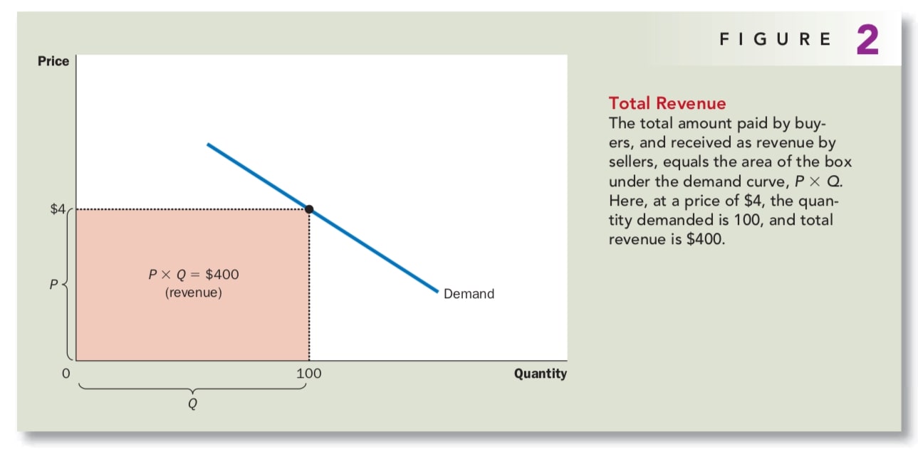
Total Revenue and The Price Elasticity of Demand
Toal revenue is the amount paid by buyers and received by sellers of the good. In any market, total revenue is P * Q, the price of the good times the quantity of the good sold. We can show total revenue graphically, as in Figure 2.
How does total revenue change as one moves along the demand curve? There are some examples in Figure 3.
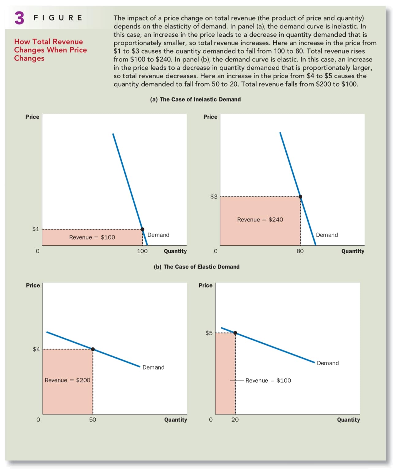
Although the examples in this figure are extreme, they illustrate some general rules:
- When demand is inelastic, price and total revenue move in the same direction.
- When demand is elastic, price and total revenue move in opposite directions.
- If demand is unit elastic (a price elasticity exactly equal to 1), total revenue remains constant when the price changes.
Elasticity and Total Revenue Along A Linear Demand Curve
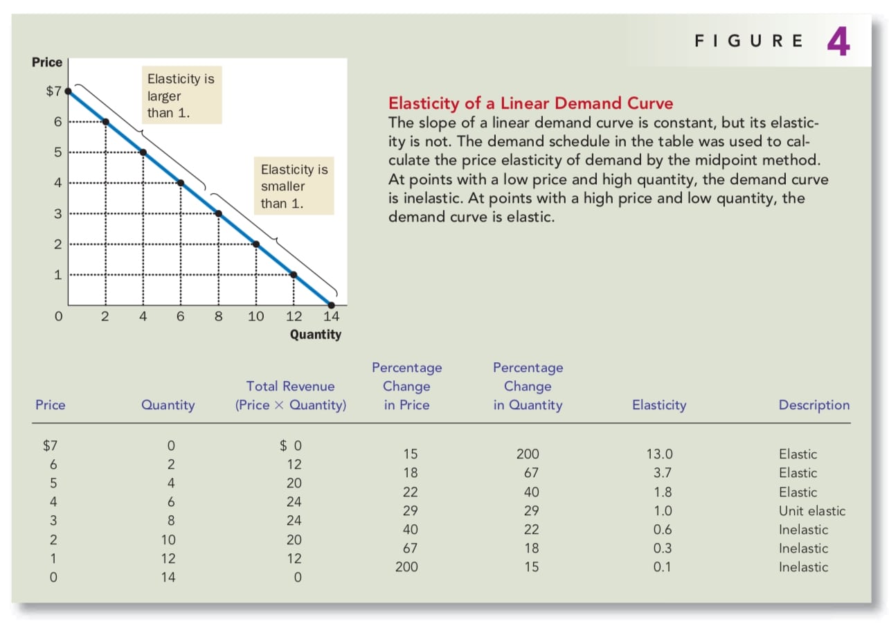
Even though the slope of a linear demand curve is constant, the elasticity is not. This is true because the slope is the ratio of changes in the two variables, whereas the elasticity is the ratio of percentage changes in the two variables. At points with a low price and high quantity, the demand curve is inelastic. At points with a high price and low quantity, the demand curve is elastic.
The linear demand curve illustrates that the price elasticity of demand need not be the same at all points on a demand curve. A constant elasticity is possible, but it is not always the case.
Other Demand Elasticities
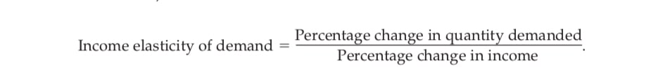
The Income Elasticity of Demand measures how the quantity demanded changes as consumer income changes.
Most of goods are normal goods: Higher income raises the quantity demanded, which have positive income elasticities. A few goods, such as bus rides, are inferior goods: Higher income lowers the quantity demanded, which have negative income elasticities.
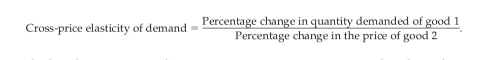
The Cross-Price Elasticity of Demand measures how the quantity demanded of one good responds to a change in the price of another good.
Substitutes are goods that are typically used in place of one another, whose cross-price elasticity is positive. Conversely, complements are goods that are typically used together, whose cross-price elasticity is negative.
The Elasticity Of Supply
The Price Elasticity of Supply And Its Determinants
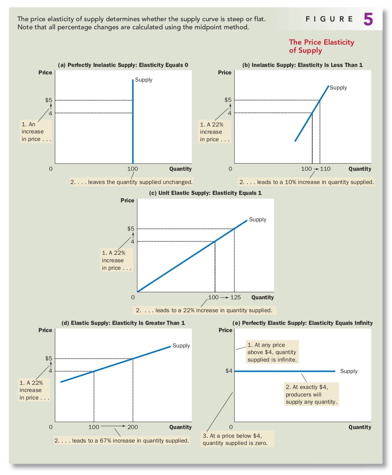
The price elasticity of supply measures how much the quantity supplied responds to changes in the price. Supply of a good is said to be elastic if the quantity supplied responds substantially to changes in the price.
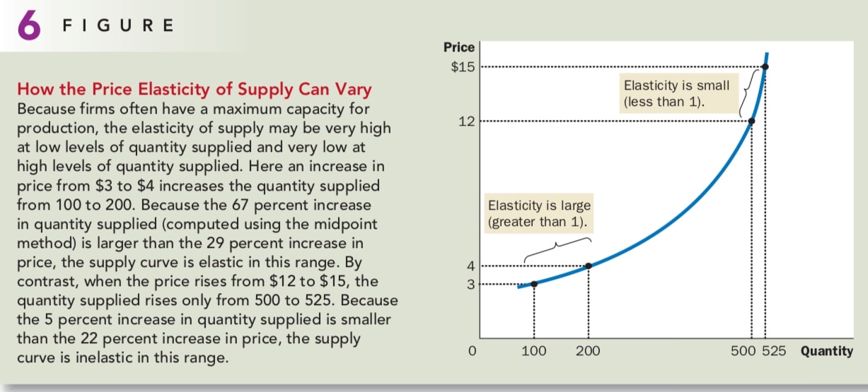
In most markets, a key determinant of the price elasticity of supply is the time period being considered. Supply is usually more elastic in the long run than in the short run.
Computing The Price Elasticity of Supply
Economists compute the price elasticity of supply as the percentage change in the quantity supplied divided by the percentage change in the price. That is, 
The Vary Of Supply Curves
Three Applications Of Supply, Demand, And Elasticity
Can Good News For Farming Be Bad News For Farmers
The raise of production provided by new farming technology could make farmers worse off. Because the new technic increase the amount of wheat that can be produced on each acre of land, farmers are willing to supply more wheat at any price. In other words, the supply curve shift to the right and the demand curve still remain the same, which cause the price of wheat falls.
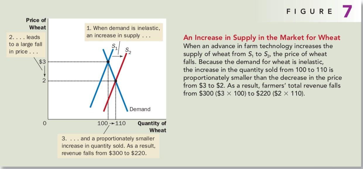
Wheat being an inelastic good, the price of wheat falls doesn’t make people buy a lot more wheat. So a decrease in price causes farmers’ total revenue to fall.
You may wonder why farmers would adopt the new technology. The answer goes to the heart of how competitive markets work. Because each farmer is only a small part of the market for wheat, it’s better to use the new technic to produce and sell more wheat at any given price. Yet when all farmers do this, the supply of wheat increases, the price falls, and farmers are worse off.
It is important to keep in mind that what is good for farmers is not necessarily good for society as a whole. Improvement in farm technology can be bad for farmers because it makes farmers increasingly unnecessary, but it is surely good for consumers who pay less for food.
Why Did OPEC Fail To Keep The Price Of Oil High?
The OPEC episode of 1970s and 1980s shows how supply and demand can behave differently in the short run and in the long run. In the short run, both the supply and demand for oil are inelastic. Supply is inelastic because the quantity of known oil reserves and the capacity for oil extraction cannot be changed quickly. Demand is inelastic because buying habits do not respond immediately to changes in price. Thus, as panel (a) of Figure 8 shows, the short-run supply and demand curves are steep.
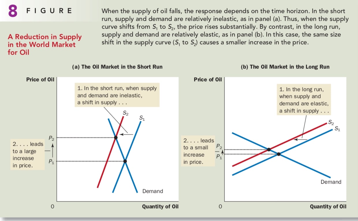
The situation is very different in the long run. Over long periods of time, producers of oil outside OPEC respond to high prices by increasing oil exploration. Consumers respond with greater conservation. Thus, as panel (b) of Figure 8 shows, the long-run supply and demand curves are more elastic.
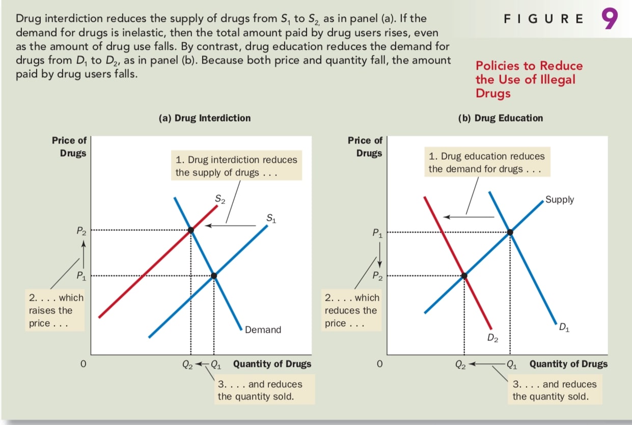
Suppose the government increase the number of federal agents devoted to the war on drugs. When the government stops some drugs from entering the country and arrests more smugglers, it raises the cost of selling drugs and, therefore, reduces the quantity of drugs supplied at any given price. But the demand for drugs is not changed, as panel (a) of Figure 9 shows.
But in terms of drug-related crime, since the demand for drugs is inelastic, then an increase in price raises total revenue in the drug market. Addicts who already had to steal to support their habits would have an even greater need for quick cash. Thus, drug interdiction could increase drug-related crime.
Rather than trying to reduce the supply of drugs, policymakers might try to reduce the demand by pursuing a policy of drug education. Successful drug education has the effects shown in panel (b) of Figure 9. Thus, in contrast to drug interdiction, drug education can reduce both drug use and drug-related crime.
However, the demand for drugs is probably inelastic over short periods, it may be more elastic elastic over longer periods because higher prices would discourage experimentation with drugs among the young and, over time, lead to fewer drug addicts. In this case, drug interdiction would increase drug-related crime in the short run while decreasing it in the long run.
The Distributional Effects of Tax
Suppose this is the supply and demand curve of the gasoline market of Chicago without tax. The market price will be ¥3 when there is no tax. So buyers pay ¥3 to buy one gallon of gasoline and sellers receive ¥3 for one gallon of gasoline.
Suppose the government imposes a tax of ¥0.5 per gallon of gasoline and suppose the buyer will pay the tax. Then the demand curve will move left because there's a tax more. And that is changing the tax everywhere in the curve. So from any point, vertically in the curve, to the other point, we're going to have a distance of 50 cents. Let’s say the new demand curve generate a new equilibrium at price ¥2.75. So, what the buyers end up paying is at ¥2.75, the buyer that goes to the Sellers, plus the 50 cents that goes to the government. So in the end, they're actually paying ¥3.25 for a gallon of gasoline.
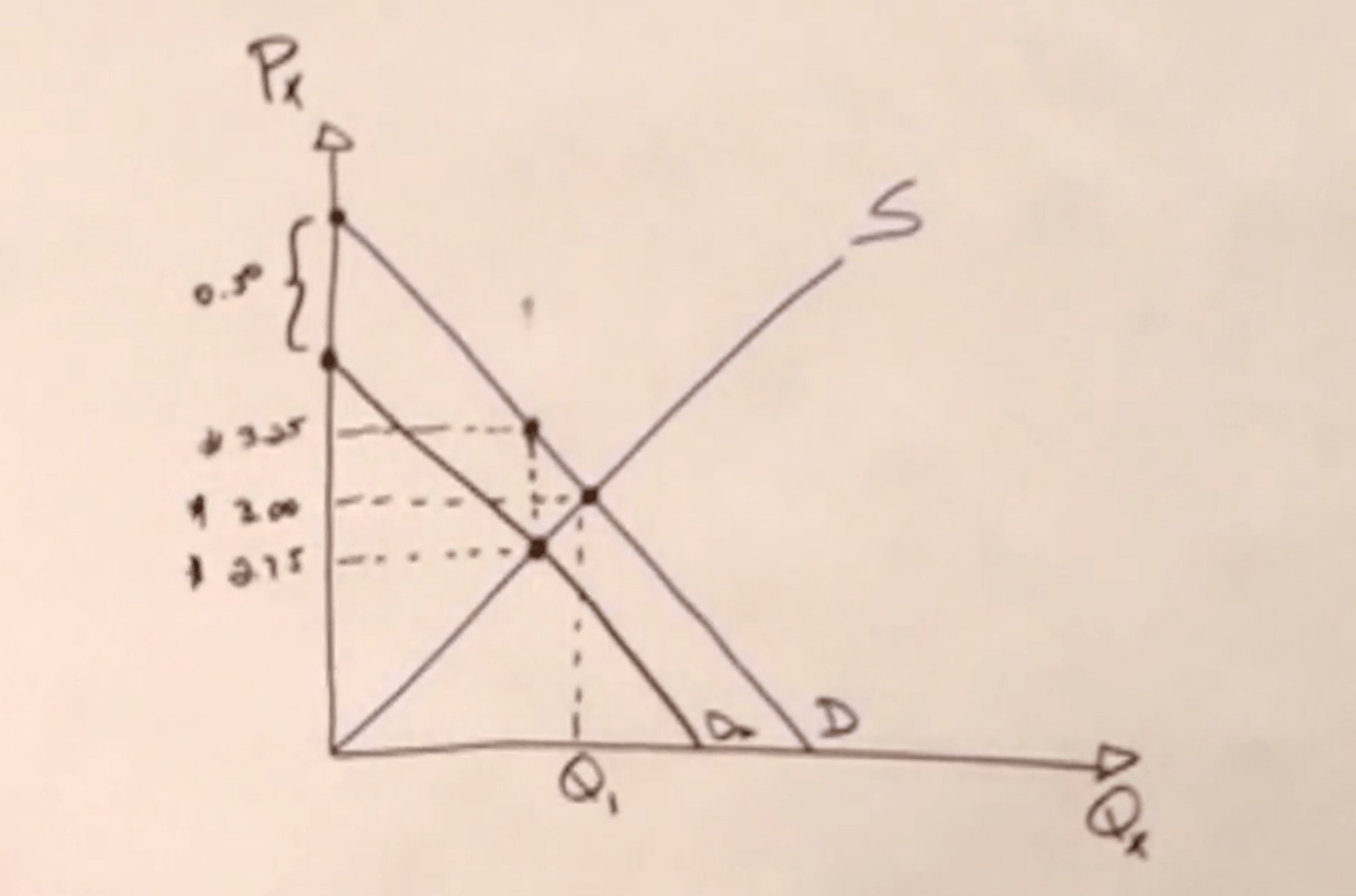
Now the buyers are paying ¥3.25. So they are worse off because they have a higher price by ¥0.25. And the sellers, while they were receiving ¥3 before, now they're only getting ¥2.75. So they are worse off by 25 cents too. Well, it looks like, in this particular situation, the buyers are sharing 25 cents, they're paying of the tax and sellers are putting up with 25 cents of the tax. So, this tax is equally distributed among the buyers and the sellers. And it doesn't matter if the sellers are the ones sending this tax to the government.
| No Tax | Tax ¥0.5 | Change | |
|---|---|---|---|
| Market Price | ¥3.00 | ¥2.75 | ¥0.25 |
| Buyers Pay | ¥3.00 | ¥3.25 | ¥0.25 |
| Sellers Receive | ¥3.00 | ¥2.75 | ¥0.25 |
So what determined the distribution of the tax is which side of the market has the most trouble adjusting to a tax. And in this particular example, we're assuming that both have the same trouble and that is based on the elasticity. And the more inclined the curve is, the more inelastic that side of the market is.
Let's say the demand curve is like that below and the supply curve is a lot flatter. So this model here makes the assumption that the demand of gasoline is more inelastic than the supply of gasoline.
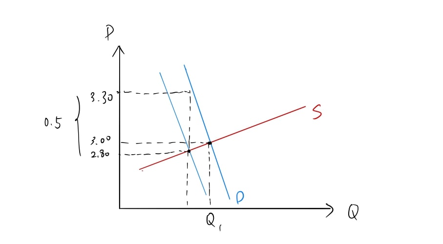
What happened? The market price went down to ¥2.80. The buyers pays ¥2.80 to the sellers, but then they pay 50 cents to the government. So they're actually paying effectively ¥3.30 with this tax. So they're paying 30 cents more than they were paying before per gallon of gasoline. How about the sellers? The sellers were selling it for ¥3 before. Now, they're getting ¥2.80 from the buyers, so they're worse off 20 cents. And it's a whole different story, because now, of the 50 cents, 30 cents are shared by the buyers and only 20 cents by the sellers. So the sellers are not sharing as much of the burden of this tax as the buyers are.
| No Tax | Tax ¥0.5 | Change | |
|---|---|---|---|
| Market Price | ¥3.00 | ¥2.80 | ¥0.20 |
| Buyers Pay | ¥3.00 | ¥3.30 | ¥0.30 |
| Sellers Receive | ¥3.00 | ¥2.80 | ¥0.20 |
So the seller has a lot more freedom here to adjust to this tax by perhaps charging a higher price to the buyers. The buyers cannot adjust as easily and they will have to put up with most of the burden. So in the end, the most inelastic side of the market is the one that actually shares most of the burden of the tax regardless of who send the tax to the government.