HKUST CSIT5401 Recognition System lecture notes 3. 识别系统复习笔记。
- Histogram Equalization
- Image Pyramid and Neural Networks
- Integral Image
- Adaboost
- Face Recognition (PCA)
Histogram Equalization
Face detection is the first step in automated face recognition. Its reliability has a major influence on the performance and usability of the entire face recognition system.
Due to lighting or shadow, intensity can vary significantly in an image. Normalization of pixel intensity helps correct variations in imaging parameters in cameras as well as changes in illumination conditions. One widely used technique is histogram equalization, which is based on image histogram. It helps reduce extreme illumination.
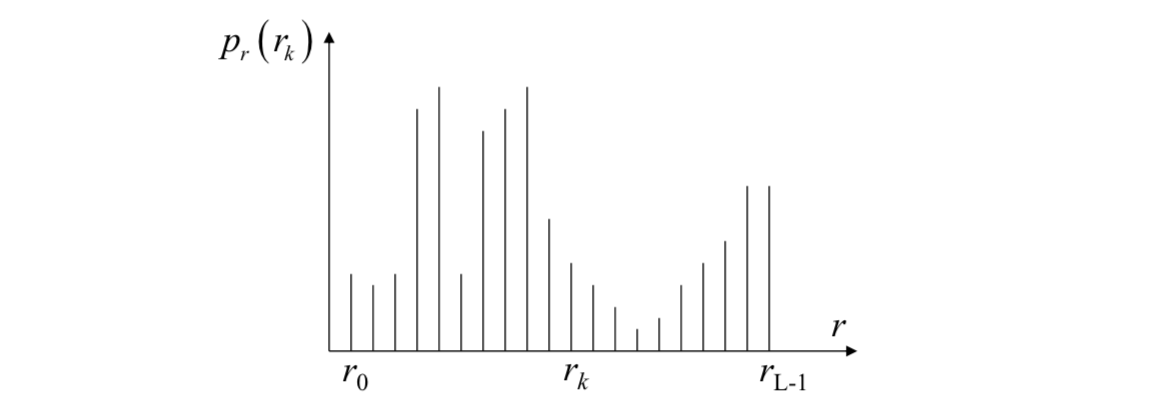
Image histogram
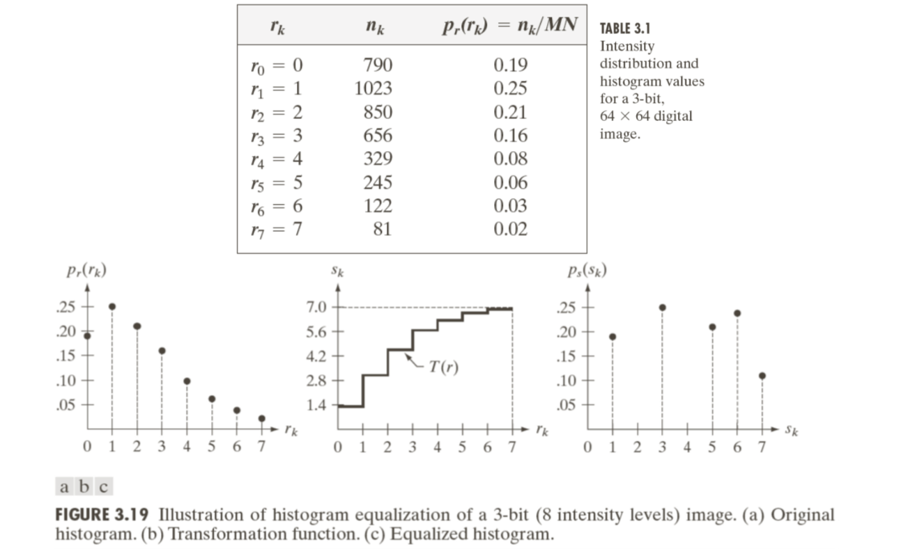
It is assumed that there is a digital image with \(L\) gray levels \(r_k\). The probability of occurrence of gray level \(r_k\) is given by \[ p_r(r_k)=\frac{n_k}{N} \] where \(n_k\) is number of pixels with gray level \(r_k\); \(N\) is total number of pixels in an image; \(k = 0,1,2,...,L-1\).
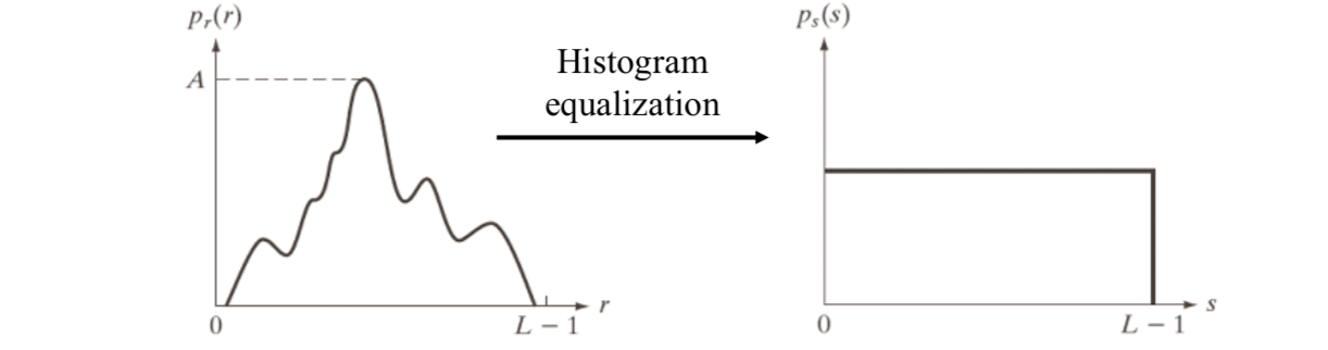
We want an image with equally many pixels at every gray level, or the output intensity approx follows uniform distribution.
That is, a flat histogram, where each gray level, \(r_k\), appears equal number of times, i.e., \(N/L\) times.
Assume that variable \(r\) has been normalized between \([0,1]\). The intensity transformation is \(s = T(r)\), such that
- \(T(r)\) is single-valued and non-decreasing in the interval \(0≤r≤1\).
- \(0≤T(r)≤1\) for \(0≤r≤1\).
Histogram equalization transform
The intensity transformation is the cumulative distribution function (CDF) of \(r\), which is represented by \[ s=T(r)=\int_0^rp_r(w)dw \] The discrete implementation is given by \[ s_k=T(r_k)=\sum_{j=0}^k\frac{n_j}{N}=\sum_{j=0}^kp_r(r_j) \] where \(s_k\) is the output intensity; \(r_k\) is the input intensity; \(n_j\) is the number of pixels with gray level \(r_j\).
Below are some examples:
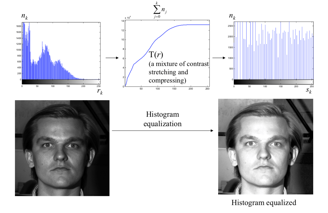
Histogram equalization can significantly improve image appearance
- Automatic
- User doesn’t have to perform windowing
Nice pre-processing step before face detection
- Account for different lighting conditions
- Account for different camera/device properties
There are two methods for face detection:
- Method using image pyramid and neural networks [Rowley-Baluja-Kanade-98]
- Method using integral image and AdaBoost learning [Viola-Jones-04]
Image Pyramid and Neural Networks
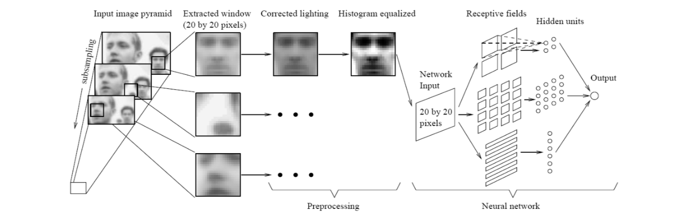
With the neural networks, a classifier may be trained directly using preprocessed and normalized face and nonface training subwindows.
Rowley et al use the preprocessed 20x20 subwindows as the input to a neural network. The final decision is made to classify the 20x20 subwindow into face and nonface. The architecture is shown below.
Instead of upright, frontal faces, a router network can be trained to process each input window so that orientation can be estimated. Once the orientation is estimated, the input window can be prepared for detector neural network.
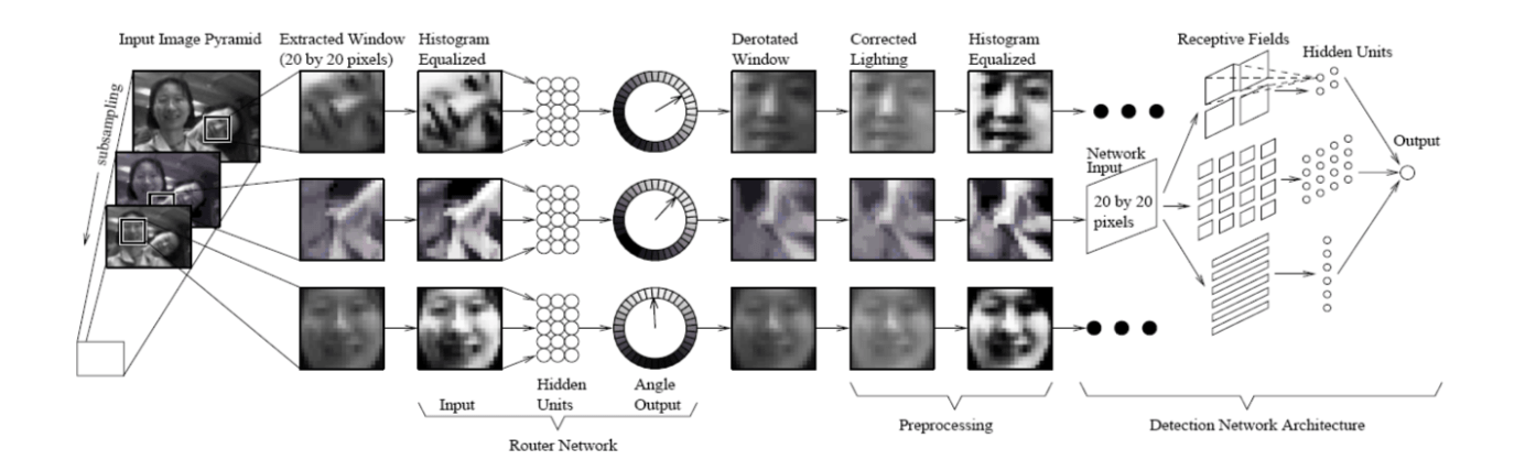
Rowley et al. proposed two neural networks, as presented in the previous slides. The first one is the router network which is trained to estimate the orientation of an assumed face in the 20x20 sub-window. The second one is the normal frontal, upright face detector. However, it only handles in-plane rotation.
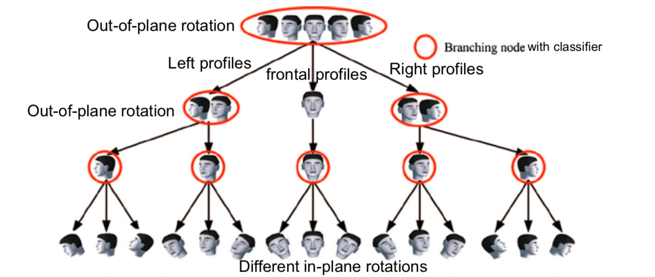
Huang et al. proposed a multi-view face tree structure for handling both in-plane and out-of-plane rotations. Every node corresponds to a strong classifier.
Integral Image
Method using integral image and AdaBoost learning
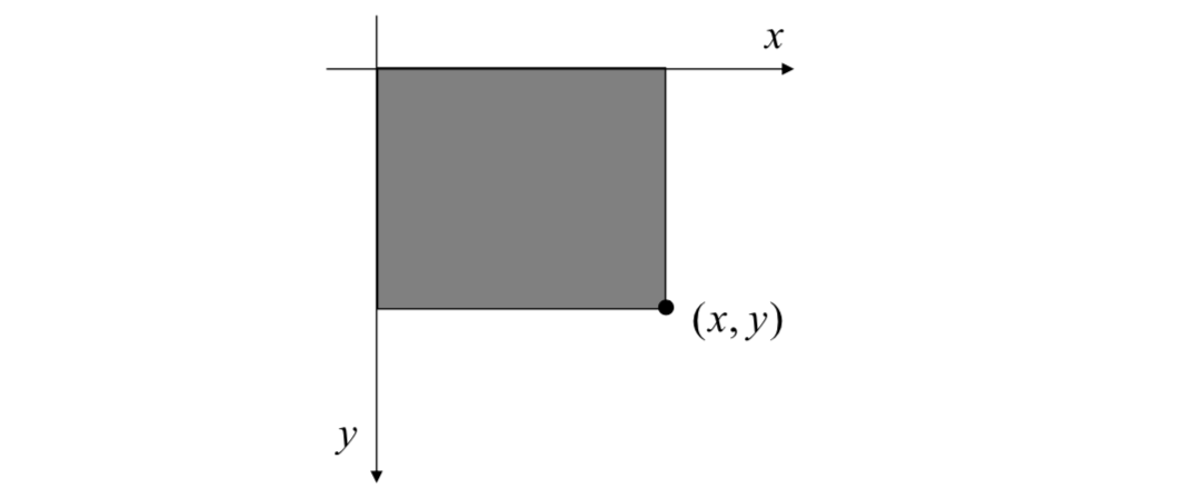
The integral image \(ii(x, y)\) at location \((x, y)\) contains the sum of the pixel intensity values above and to the left of the location \((x, y)\), inclusive.
The \(ii\) is defined as \[ ii(x,y)=\sum_{x'≤x,y'≤y}i(x',y') \] where \(ii(x,y)\) is the integral image and \(i(x,y)\) is the original input image.
Using the following pair of recurrences: \[ s(x, y)=s(x, y-1)+i(x,y)\\ ii(x,y)=ii(x-1, y)+s(x,y) \] where \(s(x,y)\) is the cumulative row sum, \(s(x, -1) = 0\), and \(ii(-1, y)=0\), the integral image can be computed in one pass over the original image.
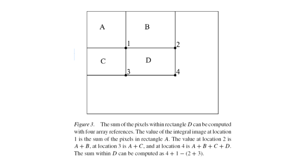
Using the integral image, any rectangular sum can be computed in four array references.
Rectangle features
The features for face detection are Haar-like functions. There are three kinds of features.
[1] Two-rectangle feature: The difference between the sum of the pixels within two rectangular regions.

[2] Three-rectangle feature: The feature is the sum within two outside rectangles subtracted from the sum in a center rectangle.

[3] Four-rectangle feature: The difference between diagonal pairs of rectangles.

The rectangle features are sensitive to the presence of edges, bars/lines, and other simple image structures in different scales and at different locations.
Given that the base resolution of the detector is 24 x 24 pixels, the exhaustive set of rectangle features is quite large, 160,000.
Given a feature set and a training set of positive and negative images, a classification function must be learned to classify a pattern into either face or non-face.
Adaboost
In this work, the classifier is designed based on the assumption that a very small number of features can be combined to form an effective classifier.
The AdaBoost learning algorithm is used to boost the classification performance of a simple learning algorithm. The simple learning algorithm is applied to all rectangle features.
It does this by combining a collection of weak classification functions (weak classifiers with relatively high classification error) to form a stronger classifier. The final strong classifier takes the form of a weighted combination of weak classifiers followed by a threshold.
Weak classifier \(h_t\) (each classifier compute one rectangle feature): \[ h_t(\vec{x})=\begin{cases} 1\ \text{if }\vec{x}\text{ represents a face image }(f_t(\vec{x})>\text{Threshold})\\ -1\ \text{otherwise} \end{cases}\\ f_t(\vec{x})=\sum_{white} x-\sum_{black} x \] The strong classifier is \[ H(\vec{x})=\text{sgn}\left(\sum_{t=1}^T\alpha_th_t(\vec{x})\right) \] where \(\alpha_t\) is weight; and \(\text{sgn}(x)\) is sign function: \[ \text{sgn}(x)=\begin{cases} -1, & \mbox{if }x≤0 \\ 1, & \mbox{if }x>0 \end{cases} \] Algorithm
Given example images and classifications \((\vec{x}_i, y_i), i = 1, 2,..., N\), where \(N\) is the total number of images.
Start with equal weights on each image \(\vec{x}_i\).
For \(t=1, ..., T\):
Normalize all weights \(w_i = \frac{w_i}{\sum_{j=1}^Nw_j}\) such that \(\sum_{i=1}^Nw_i=1\).
Select the weak classifier \(h_k\) with minimum error: \[ e_k=\sum_{i=1}^Nw_i\left(\frac{1-h_k(\vec{x}_i)y_i}{2}\right) \] where \(0≤e_k≤1\).
Set weight for selected weak classifier \[ \alpha_t=\frac{1}{2}\ln\left(\frac{1-e_k}{e_k}\right) \]
Reweight the examples (boosting) \[ w_i=w_i\exp(-\alpha_iy_ih_k(\vec{x}_i)) \]
For the last step, if the weak classifier classify example \(i\) correctly, i.e. \(h_k(\vec{x}_i)=y_i\), then the example weight \(w_i=w_ie^{-\alpha_t}\) will decrease; if the weak classifier classify example \(i\) wrongly, the weight \(w_i=w_i^{\alpha_t}\) will increase.
Values of \(T\) can be 200 for \(N=10^8\) images and 180,000 filters. Given the above strong classifier, a new image can classified as either face or non-face.
Face Recognition (PCA)
Images of faces often belong to a manifold of intrinsically low dimension. For example, if there are three 3x1 images (see below), then each image has three intensity values. If each intensity value is viewed as a coordinate in a 3D space, then each image can be viewed as a point in a 3D space.
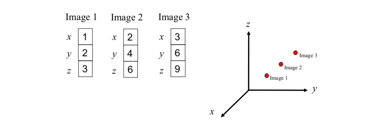
To represent these points effectively, the number of dimensions can be reduced from three to one. It is the concept of dimensionality reduction.
Principal component analysis (PCA) is a method for performing dimensionality reduction of high dimensional face images.
Eigenfaces
Let us consider a set of \(N\) sample images (image vectors) with \(m\times n\) dimensions:

Each image is represented by a 1D vector with dimensions \((m\times n) \times 1\). The mean image vector is given by \[ \vec{x}=\frac{1}{N}\sum_{i=1}^N\begin{bmatrix} x_{i,1} \\ \vdots \\ x_{i,mn} \end{bmatrix} \] The scatter matrix is given by \[ \vec{S}=[\vec{x_1}-\bar{x}\ \ \vec{x_2}-\bar{x}\ \dots\ \vec{x_N}-\bar{x}]\begin{bmatrix} (\vec{x_1}-\bar{x})^T \\ (\vec{x_2}-\bar{x})^T\\ \vdots \\ (\vec{x_N}-\bar{x})^T \end{bmatrix} \] The corresponding \(t\) eigenvectors with non-zero eigenvalues \(\lambda_i\) are \[ \vec{e}_1\ \ \vec{e}_2\ \ \dots\ \ \vec{e}_t \] where \(\lambda_1≥\lambda_2≥...≥\lambda_t\).
Then the origin image vector can be approximated by \[ \vec{x}_j\approx\bar{x}+\sum_{i=1}^tg_{ji}\vec{e}_i \] where \(g_{ji}=(\vec{x}_j-\bar{x})\cdot\vec{e}_i\).
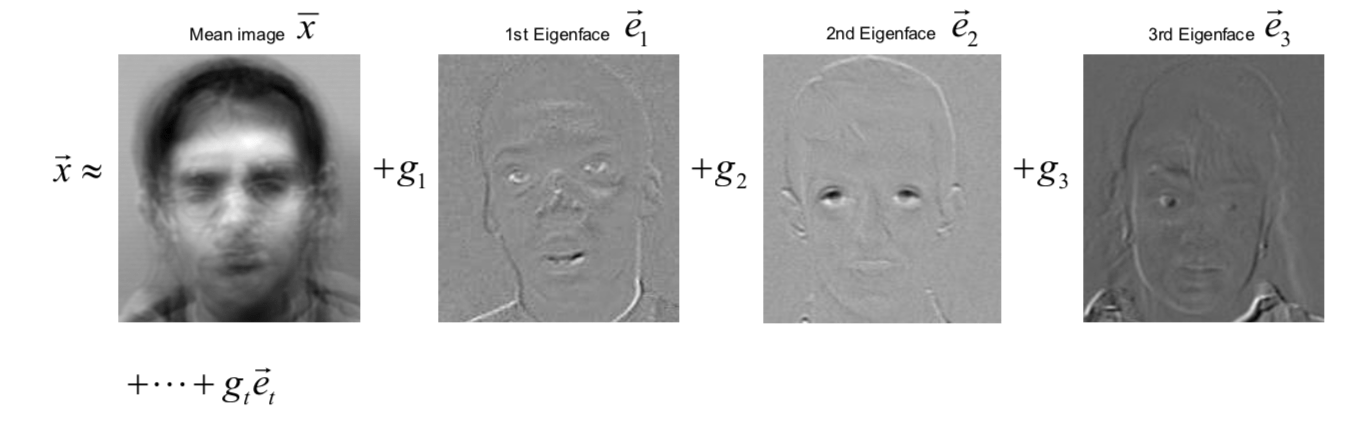
Since the eigenvectors \(e\) have the same dimension as the image vectors, the eigenvectors are referred as Eigenfaces. The value of \(t\) is usually much smaller than the value of \(mn\). Therefore, the number of dimensions can be reduced significantly.
For each image \(\vec{x}_i\), the dimension reduced representation is \[ (g_{i1}, g_{i2}, ..., g_{it}) \] To detect if the new image \(\vec{x}\) with \(t\) coefficients \((g_1, g_2, ..., g_t)\) is a face: \[ ||\vec{x}-(\bar{x}+g_1\vec{e}_1+g_2\vec{e}_2+...+g_t\vec{e}_t)||<\text{Threshold} \] If it is a face, find the closest labeled face based on the nearest neighbor in the \(t\)-dimensional space.
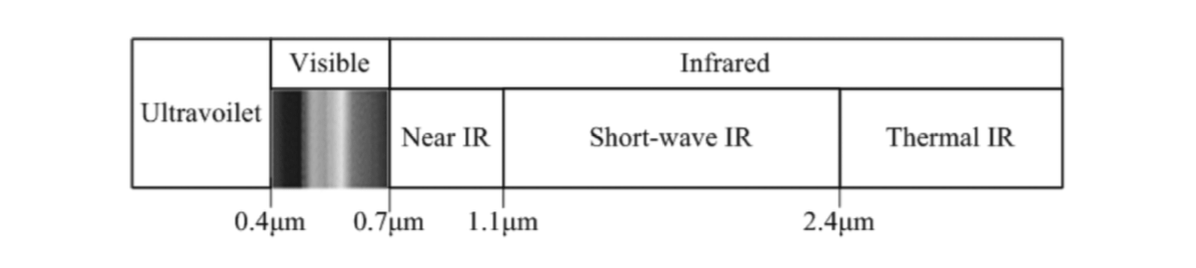
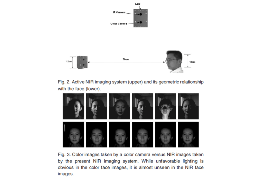
Near-infrared images for face recognition
Most current face recognition systems are based on face images captured in the visible light spectrum. The infrared imaging system is able to produce face images of good condition regardless of visible lights in the environment.