Introduction
Last lecture, David taught us how to solve a known MDP, which is planning by dynamic programming. In this lecture, we will learn how to estimate the value function of an unknown MDP, which is model-free prediction. And in the next lecture, we will optimise the value function of an unknown MDP.
In summary:
- Planning by dynamic programming
- Solve a known MDP
- Model-Free prediction
- Estimate the value function of an unknown MDP
- Model-Free control
- Optimise the value function of an unknown MDP
We have two major methods to estimate the value function of an unknown MDP:
- Monte-Carlo Learning
- Temporal-Difference Learning
We will introduce the two methods and combine them to a general method.
Table of Contents
Monte-Carlo Learning
MC (Monte-Carlo) methods learn directly from episodes of experience, which means:
- MC is model-free: no knowledge of MDP transitions / rewards
- MC learns from complete episodes: no bootstrapping
- MC uses the simplest possible idea: value = mean return
- Can only apply MC to episodic MDPs: all episodes must terminate
Goal: learn \(v_\pi\) from episodes of experience under policy \(\pi\) \[ S_1, A_1, R_2, ..., S_k \sim \pi \] Recall that the return is the total discounted reward: \[ G_t = R_{t+1}+\gamma R_{t+2} + ... + \gamma^{T-1}R_T \] Recall that the value function is the expected return: \[ v_\pi(s) = \mathbb{E}_\pi[G_t|S_t=s] \] Monte-Carlo policy evaluation uses empirical mean return instead of expected return.
First-Visit Monte-Carlo Policy Evaluation
To evaluate state \(s\), the first time-step \(t\) that state \(s\) is visited in an episode:
- Increment counter \(N(s) \leftarrow N(s) + 1\)
- Increment total return \(S(s) \leftarrow S(s) + G_t\)
Value is estimated by mean return \(V(s) = S(s) / N(s)\), by law of large numbers, \(V(s) \rightarrow v_\pi(s)\) as \(N(s) \rightarrow \infty\).
Every-Visit Monte-Carlo Policy Evaluation
To evaluate state \(s\), every time-step \(t\) that state \(s\) is visited in an episode:
- Increment counter \(N(s) \leftarrow N(s) + 1\)
- Increment total return \(S(s) \leftarrow S(s) + G_t\)
Value is estimated by mean return \(V(s) = S(s) / N(s)\). Again, by law of large numbers, \(V(s) \rightarrow v_\pi(s)\) as \(N(s) \rightarrow \infty\).
Blackjack Example
Please refer to https://www.wikiwand.com/en/Blackjack to learn the rule of Blackjack.
If we build an RL agent to play blackjack, the states would have 3-dimension:
- Current sum (12 - 21)
- We just consider this range because if the current sum is lower than 12, we will always take another card.
- Dealer's showing card (ace - 10)
- Do I have a "useable" ace? (yes - no)
So there would be 200 different states.
The actions are:
- Stick: stop receiving cards and terminate
- Twist: take another card (no replacement)
And reward for action
- Stick
- \(+1\) if sum of cards \(>\) sum of dealer cards
- \(0\) if sum of cards \(=\) sum of dealer cards
- \(-1\) if sum of cards \(<\) sum of dealer cards
- Twist
- \(-1\) if sum of cards \(> 21\) and terminate
- \(0\) otherwise
Transitions: automatically twist if sum of cards < 12.
Policy: stick if sum of cards \(≥ 20\), otherwise twist.
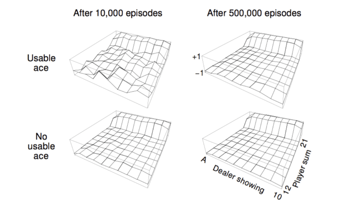
In the above diagrams, the height represents the value function of that point. Since it's a simple policy, the value funtion achieves high value only if player sum is higher than 20.
Incremental Mean
The mean \(\mu_1, \mu_2, …\) of a sequence \(x_1, x_2, …\) can be computed incrementally, \[ \begin{align} \mu_k & = \frac{1}{k}\sum^k_{j=1}x_j \\ & = \frac{1}{k}(x_k+\sum^{k-1}_{j=1}x_j) \\ &= \frac{1}{k}(x_k+(k-1)\mu_{k-1}) \\ &= \mu_{k-1}+\frac{1}{k}(x_k-\mu_{k-1}) \\ \end{align} \] which means the current mean equals to previous mean plus some error. The error is \(x_k - \mu_{k-1}\) and the step-size is \(\frac{1}{k}\), which is dynamic.
Incremental Monte-Carlo Updates
Update \(V(s)\) incrementally after episode \(S_1, A_1, R_2, …, S_T\), for each state \(S_t\) with return \(G_t\), \[ N(S_t) \leftarrow N(S_t) + 1 \]
\[ V(S_t)\leftarrow V(S_t)+\frac{1}{N(S_t)}(G_t-V(S_t)) \]
In non-stationary problems, it can be useful to track a running mean, i.e. forget old episodes, \[ V(S_t)\leftarrow V(S_t) + \alpha(G_t-V(S_t)) \] So, that's the part for Monte-Carlo learning. It's a very simple idea: you run out an episode, look the complete return and update the mean value of the sample return for each state you have visited.
Temporal-Difference Learning
Temporal-Difference (TD) methods learn directly from episodes of experiences, which means
- TD is model-free: no knowledge of MDP transitions / rewards
- TD learns from incomplete episodes, by bootstrapping. (A major difference from MC method)
- TD updates a guess towards a guess.
Goal: learn \(v_\pi\) online from experience under policy \(\pi\).
Incremental every-visit Monte-Carlo
- Update value \(V(S_t)\) toward actual return \(\color{Red}{G_t}\) \[ V(S_t)\leftarrow V(S_t)+\alpha (\color{Red}{G_t}-V(S_t)) \]
Simplest temporal-difference learning algorithm: TD(0)
Update value \(V(S_t)\) towards estimated return \({\color{Red}{R_{t+1}+\gamma V(S_{t+1})}}\) \[ V(S_t)\leftarrow V(S_t)+ \alpha ({\color{Red}{R_{t+1}+\gamma V(S_{t+1})}}-V(S_t)) \]
\(R_{t+1}+\gamma V(S_{t+1})\) is called the TD target;
\(\delta = R_{t+1}+\gamma V(S_{t+1})-V(S_t)\) is called the TD error.
Let's see a concret driving home example.
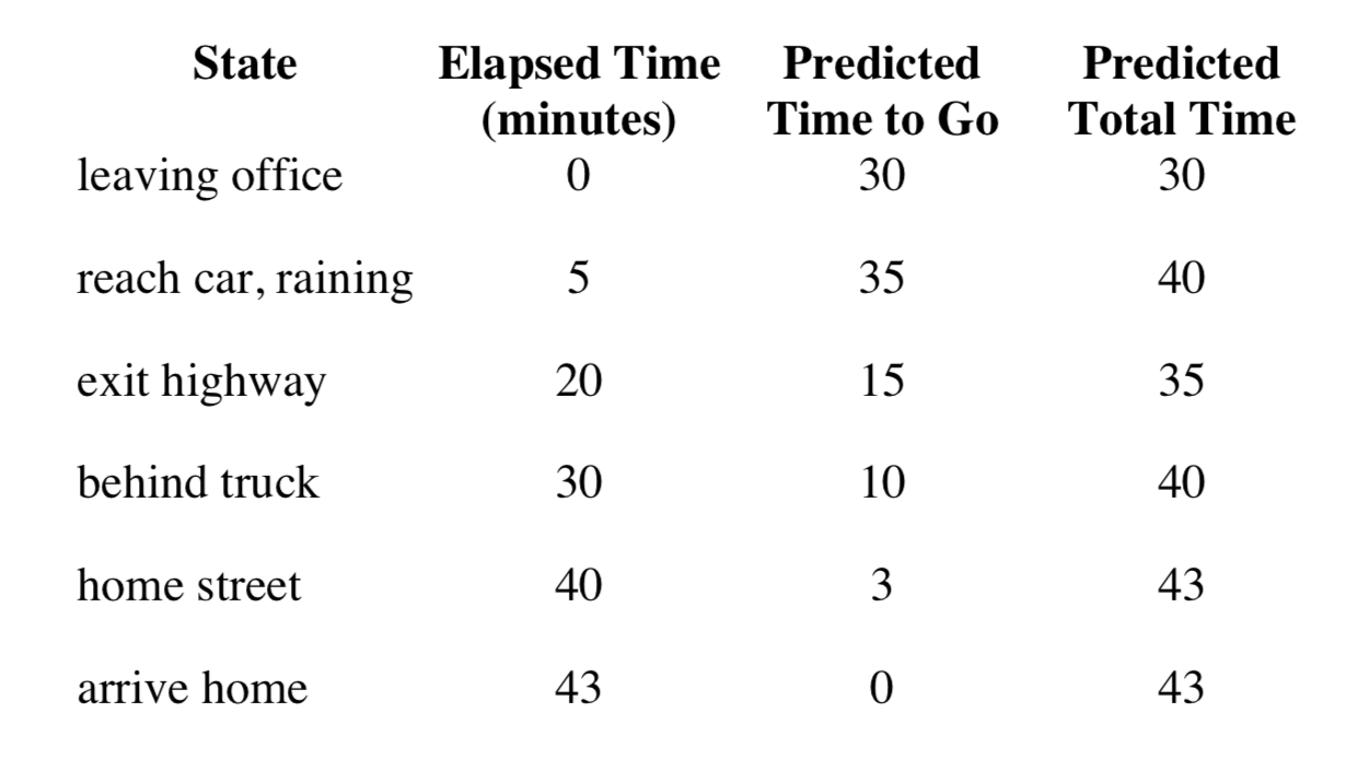
The Elapsed Time shows the actual time that has spent, the Predicted Time to Go represents the predicted time to arrive home from current state, and the Predicted Total Time means the predicted time to arrive home from leaving office.
Advantages and Disadvantages of MC vs. TD
TD can learn before knowing the final outcome
- TD can learn online after every step
- MC must wait until end of episode before return is known
TD can learn without the final outcome
- TD can learn from incomplete sequences
- MC can only learn from complete sequences
- TD works in continuing (non-terminating) environments
- MC only works for episodic (terminating) environments
MC has high variance, zero bias
- Good convergence properties (even with function approximation)
- Not very sensitive to initial value
- Very simple to understand and use
TD has low variance, some bias
- Usually more efficient than MC
- TD(0) converges to \(v_\pi(s)\) (but not always with function approximation)
- More sensitive to initial value
Bias/Variance Trade-Off
Return \(G_t = R_{t+1} + \gamma R_{t+2}+…+\gamma^{T-1}R_T\) is unbiased estimate of \(v_\pi(S_t)\).
True TD target \(R_{t+1}+\gamma v_\pi(S_{t+1})\) is unbiased estimate of \(v_\pi(S_t)\)
Explanation of bias and variance:
- The bias of an estimator is the difference between an estimator's expected value and the true value of the parameter being estimated.
- A variance value of zero indicates that all values within a set of numbers are identical; all variances that are non-zero will be positive numbers. A large variance indicates that numbers in the set are far from the mean and each other, while a small variance indicates the opposite. Read more: Variance
While TD target \(R_{t+1}+\gamma V(S_{t+1})\) is biased estimate of \(v_\pi(S_t)\).
However, TD target is much lower variance than the return, since
- Return depends on many random actions, transitions, rewards
- TD target depends on one random actions, transition, reward
Random Walk Example
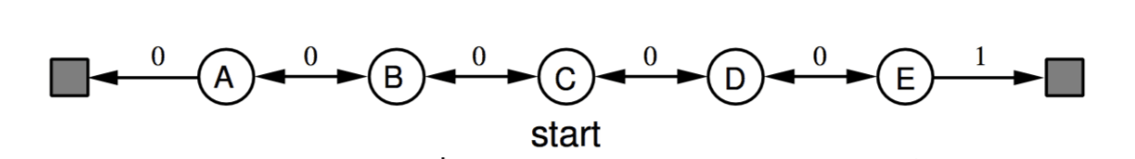
There are several states on a street, the black rectangles are terminate states. Each transition has 0.5 probability and the reward is marked on the line. The question is what is the value function of each state?
Using TD to solve the problem:
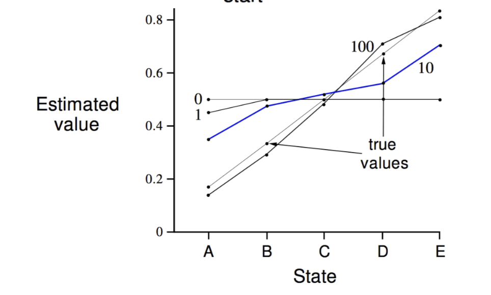
The x-axis represents each state, y-axis represent the estimated value. Each line represents the result of TD algorithm that run different episodes. We can see, at the begining, all states have initial value \(0.5\). After 100 episodes, the line converges to diagonal, which is the true values.
Using MC to solve the problem:
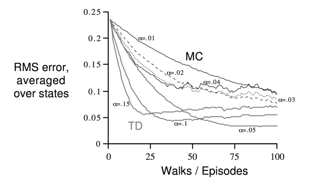
The x-axis represents the number of episodes that algorithm takes. The y-axis shows the error of the algorithm. The black lines shows using MC methods with different step-size, while the grey lines below represents using TD methods with different step-size. We can see TD methods are more efficient than MC methods.
Batch MC and TD
We know that MC and TD converge: \(V(s) \rightarrow v_\pi(s)\) as experience \(\rightarrow \infty\). But what about batch solution for finite experience? If we repeatly train some finite sample episodes with MC and TD respectively, do the two algorithms give same result?
AB Example
To get more intuition, let's see the AB example.
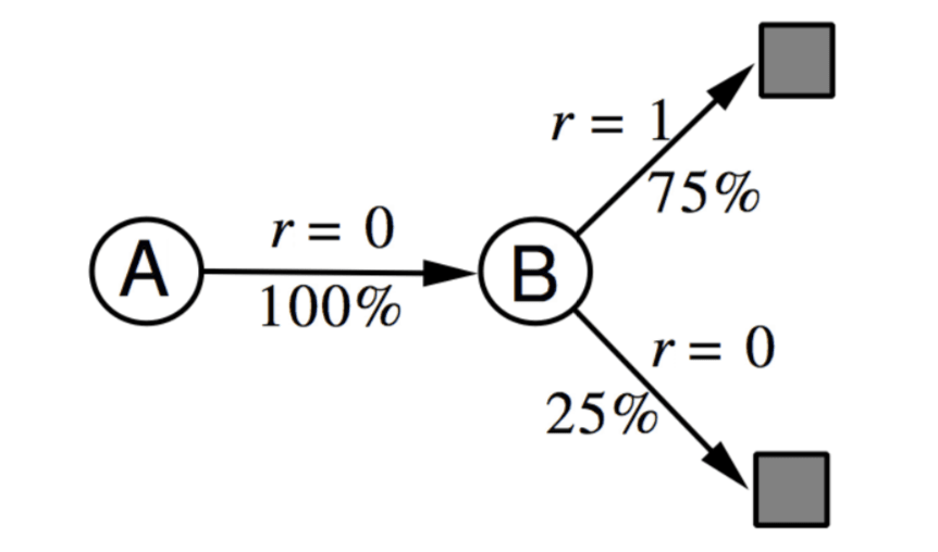
There are two states in a MDP, \(A, B\) with no discounting. And we have 8 episodes of experience:
- A, 0, B, 0
- B, 1
- B, 1
- B, 1
- B, 1
- B, 1
- B, 1
- B, 0
For example, the first episode means we in state \(A\) and get \(0\) reward, then transit to state \(B\) getting \(0\) reward, and then terminate.
So, What is \(V(A), V(B)\) ?
First, let's consider \(V(B)\). \(B\) state shows 8 times and 6 of them get reward \(1\), 2 of them get reward \(0\). So \(V(B) = \frac{6}{8} = 0.75\) according to TD and MC.
However, if we consider \(V(A)\), MC method will give \(V(A) = 0\), since \(A\) just shows in one episode and the reward of that episode is \(0\). TD method will give \(V(A) = 0 + V(B) = 0.75\).
The MDP of these experiences can be illustrated as
Certainty Equivalence
As we show above,
MC converges to solution with minimum mean-squared error
Best fit to the observed returns \[ \sum^K_{k=1}\sum^{T_k}_{t=1}(G^k_t-V(s^k_t))^2 \]
In the AB example, \(V(A) = 0\)
TD(0) converges to solution of max likelihood Markov model
Solution to the MDP \(<\mathcal{S, A, P, R, }\gamma>\) that best fits the data
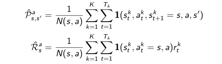
(First, count the transitions. Then compute rewards.)
In the AB example, \(V(A) = 0.75\)
Advantages and Disadvantages of MC vs. TD (2)
- TD exploits Markov property
- Usually more efficient in Markov environments
- MC does not exploit Markov property
- Usually more effective in non-Markov environments
Unified View
Monte-Carlo Backup
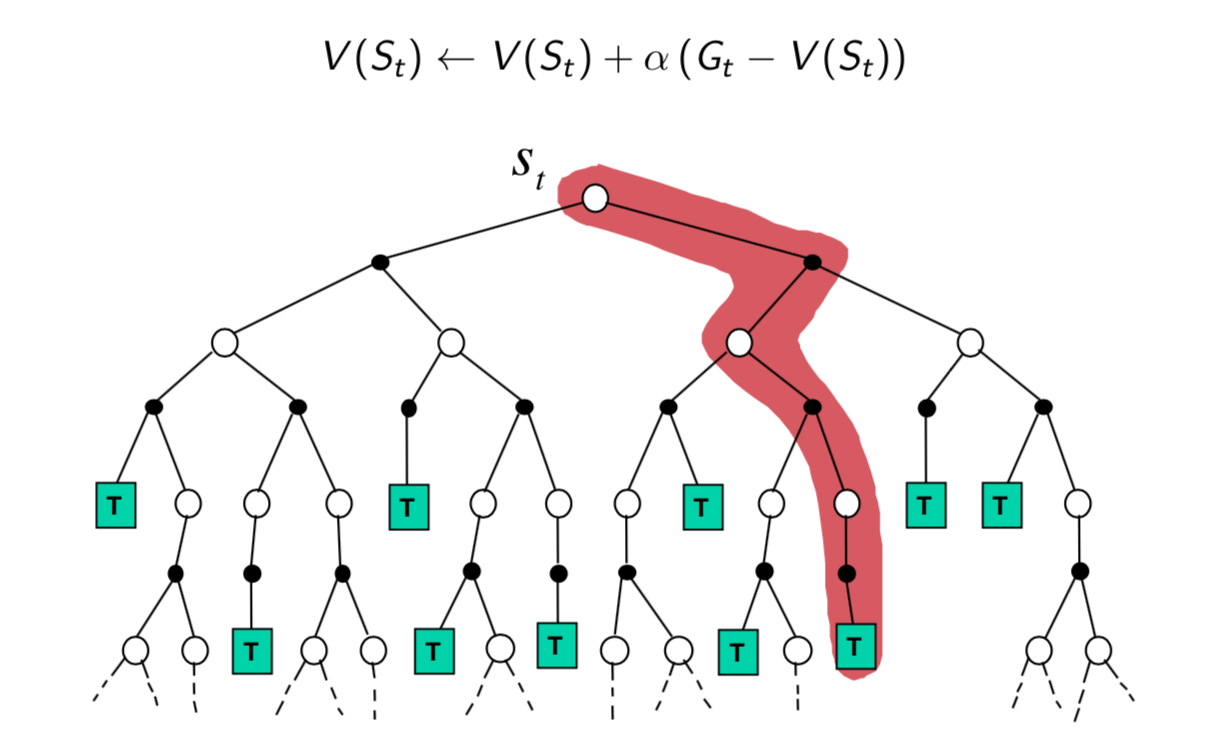
We start from \(S_t\) to look-ahead and build a look-ahead tree. What Monte-Carlo do is to sample a episode until it terminates and use the episode to update the value of state \(S_t\).
Temporal-Difference Backup
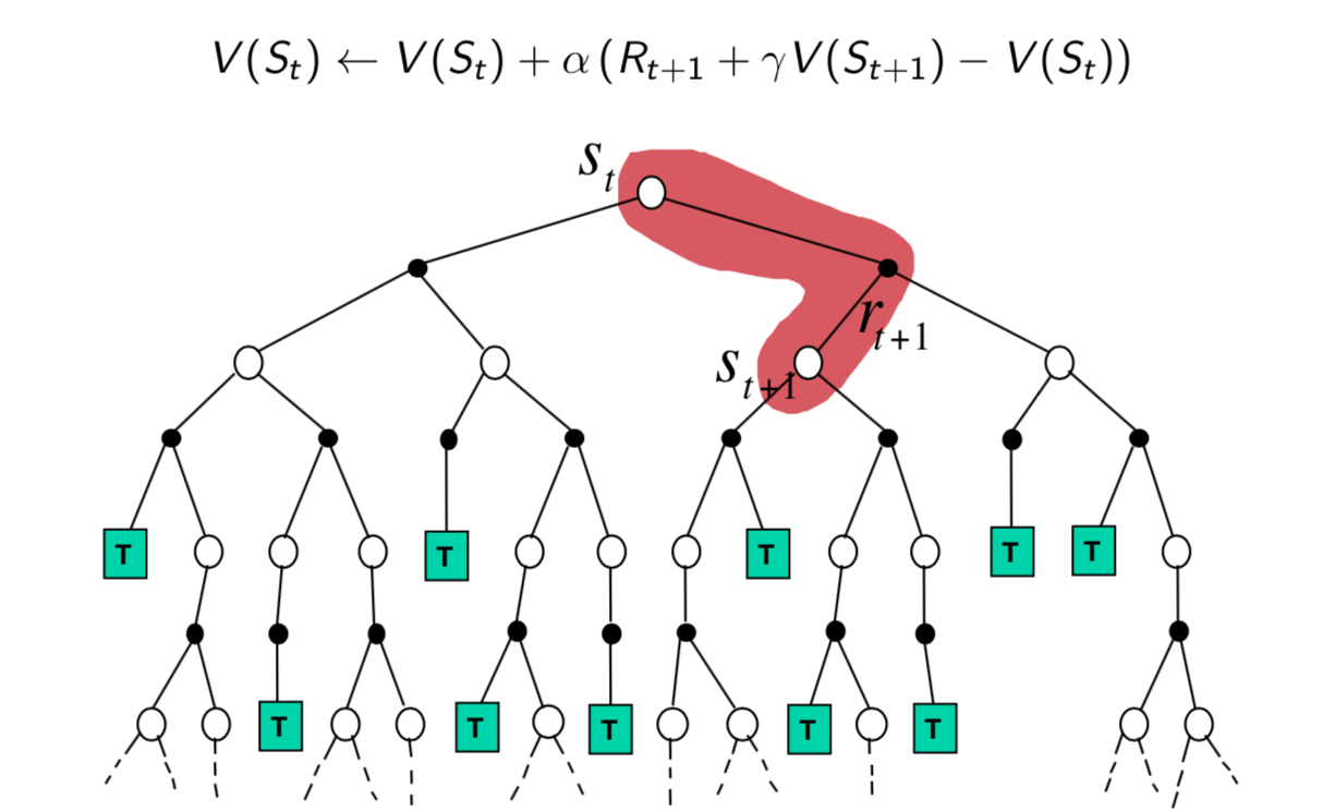
On the contrary, TD backup just sample one-step ahead and use the value of \(S_{t+1}\) to update \(S_t\).
Dynamic Programming Backup
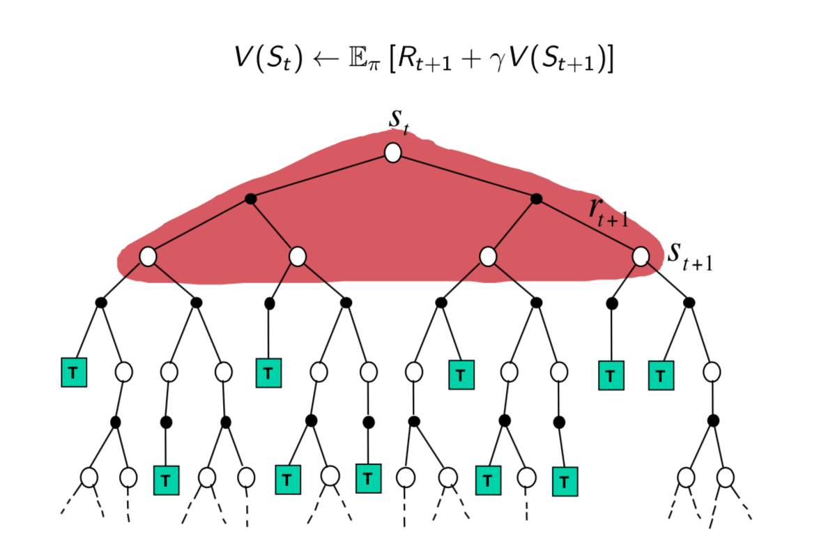
In dynamic programming backup, we do not sample. Since we know the environment, we look all possible one-step ahead and weighted them to update the value of \(S_t\).
Bootstrapping and Sampling
- Bootstrapping: update involves an estimate
- MC does not bootstrap
- DP bootstraps
- TD bootstraps
- Sampling: update samples an expectation
- MC samples
- DP does not sample
- TD samples
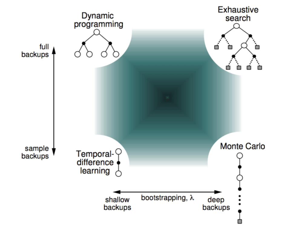
Unified View of Reinforcement Learning
TD(\(\lambda\))
Let TD target look \(n\) steps into the future,
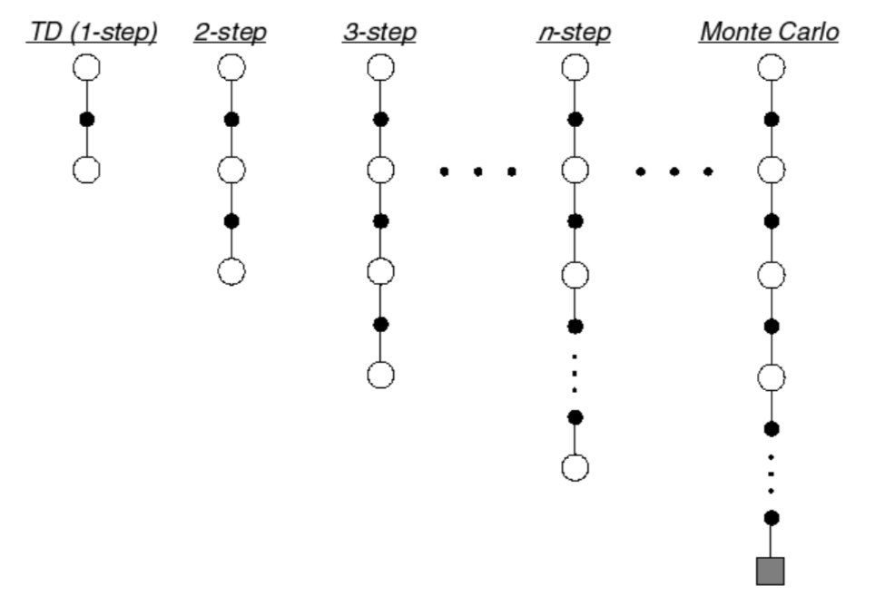
Consider the following \(n\)-step returns for \(n = 1, 2, …, \infty\):
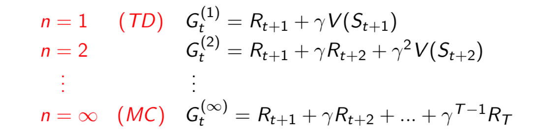
Define the \(n\)-step return \[ G_t^{(n)} = R_{t+1}+\gamma R_{t+2}+...+\gamma^{n-1}R_{t+n}+\gamma^n V(S_{t+n}) \] \(n\)-step temporal-difference learning: \[ V(S_t)\leftarrow V(S_t)+\alpha (G_t^{(n)}-V(S_t)) \] We know that \(n \in [1, \infty)\), but which \(n\) is the best?
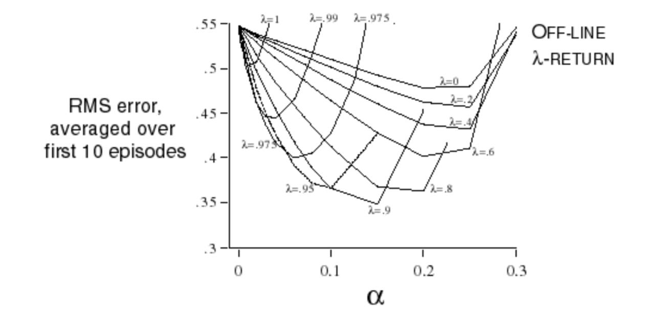
There are some experiments about that:
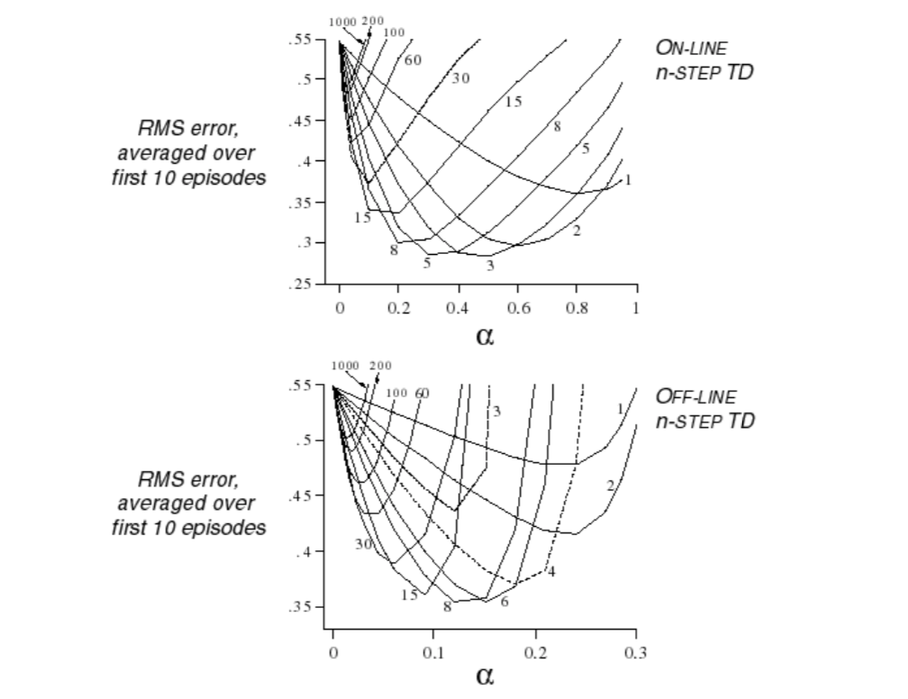
So, you can see that the optimal \(n\) changes with on-line learning and off-line leanring. If the MDP changes, the best \(n\) also changes. Is there a robust algorithm to fit any different situation?
Forward View TD(\(\lambda\))
Averaging n-step Returns
We can average n-step returns over different \(n\), e.g. average the 2-step and 4-step returns: \[ \frac{1}{2}G^{(2)}+\frac{1}{2}G^{(4)} \] But can we efficiently combine information from all time-steps?
The answer is yes.
\(\lambda\)-return
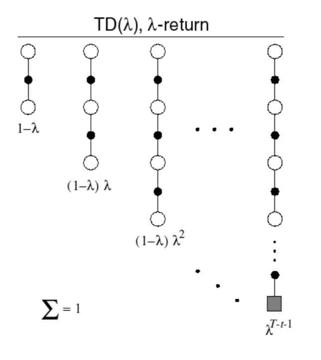
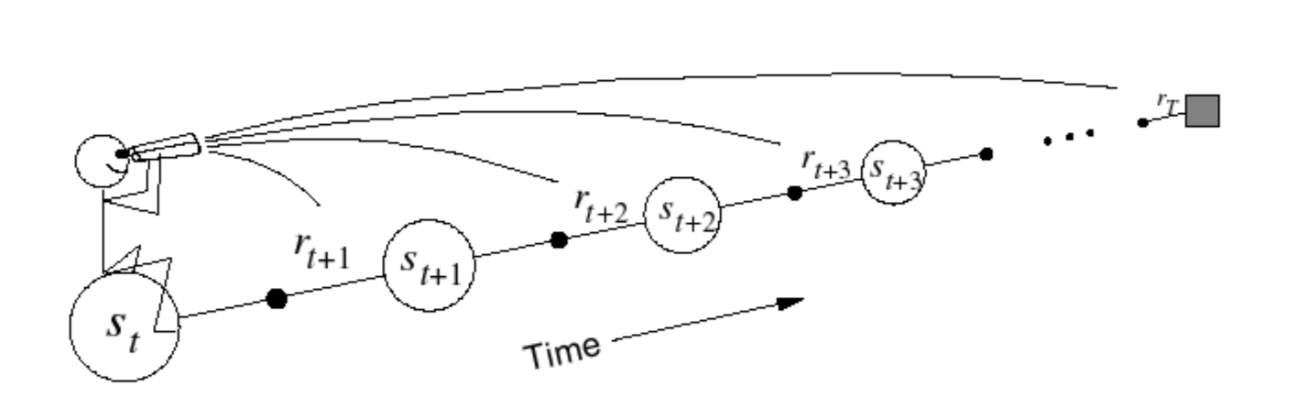
The \(\lambda\)-return \(G_t^{\lambda}\) combines all n-step returns \(G_t^{(n)}\) using weight \((1-\lambda)\lambda^{n-1}\): \[
G_t^\lambda = (1-\lambda)\sum^\infty_{n=1}\lambda^{n-1}G_t^{(n)}
\] Forward-view \(TD(\lambda)\), \[
V(S_t) \leftarrow V(S_t) + \alpha (G_t^\lambda-V(S_t))
\] 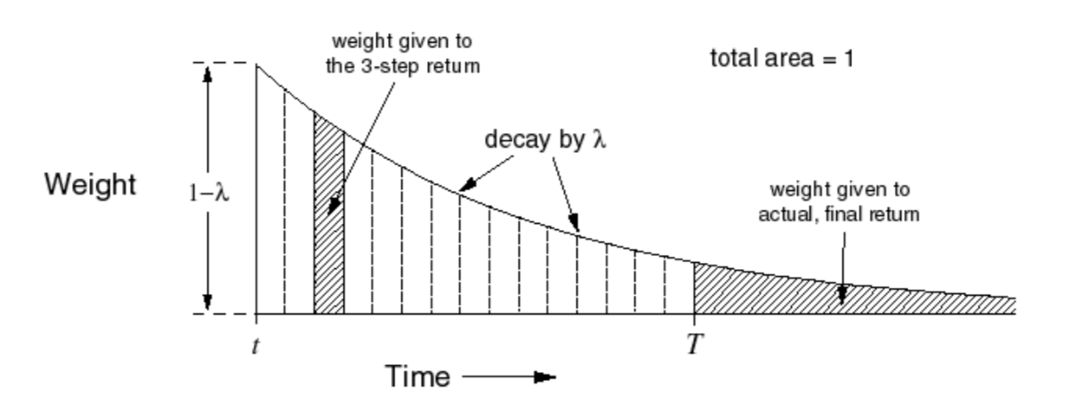
We can see the weight decay geometrically and the weights sum to 1.
The reason we use geometrical decay rather than other weight because it's efficient to compute, we can compute TD(\(\lambda\)) as efficient as TD(0).
Forward-view \(TD(\lambda)\)
- Updates value function towards the \(\lambda\)-return
- Looks into the future to compute \(G_t^\lambda\)
- Like MC, can only be computed from complete episodes
Backward View TD(\(\lambda\))
Eligibility Traces

Recall the rat example in lecture 1, credit assignment problem: did bell or light cause shock?
- Frequency heuristic: assign credit to most frequent states
- Recency heuristic: assign credit to most recent states
Eligibility traces combine both heuristics.
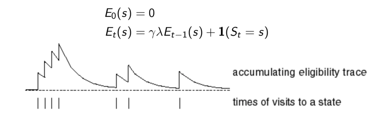
If visit state \(s\), \(E_t(s)\) plus \(1\); otherwise \(E_t(s)\) decay exponentially.
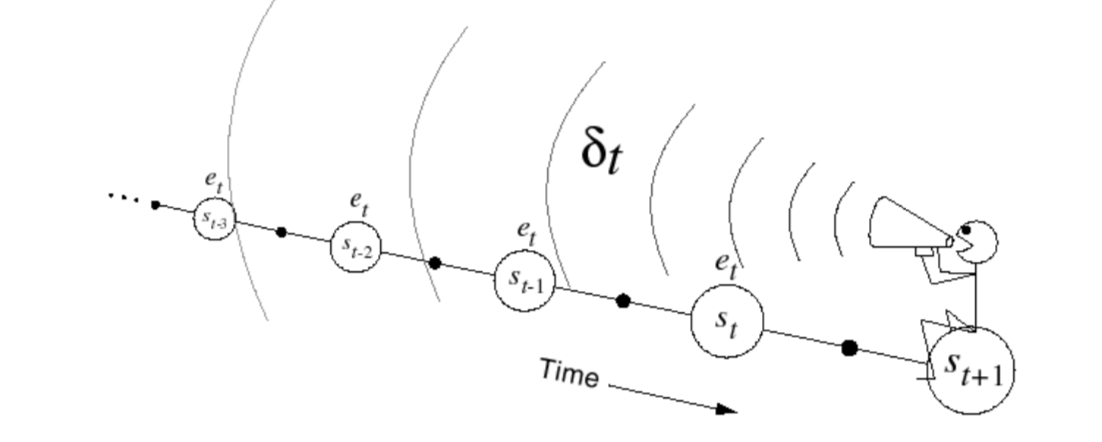
Backward View TD(\(\lambda\))
- Keep an eligibility trace for every state \(s\)
- Update value \(V(s)\) for every state \(s\) in proportion to TD-error \(\delta_t\) and eligibility trace \(E_t(s)\)
\[ \delta_t=R_{t+1}+\gamma V(S_{t+1})-V(S_t) \]
\[ V(s)\leftarrow V(s)+\alpha \delta_tE_t(s) \]
When \(\lambda = 0\), only current state is updated, which is exactly equivalent to TD(0) update: \[ E_t(s) = 1(S_t = s) \]
\[ V(s)\leftarrow V(s)+\alpha\delta_tE_t(s) = V(S_t)+\alpha\delta_t \]
When \(\lambda = 1\), credit is deferred until end of episode, total update for TD(1) is the same as total update for MC.
Relationship Between Forward and Backward TD
Theorem
The sum of offline updates is identical for forward-view and backward-view TD(\(\lambda\)) \[ \sum^T_{t=1}\alpha\delta_tE_t(s)=\sum^T_{t=1}\alpha(G_t^\lambda-V(S_t))1(S_t=s) \]
MC and TD(1)
Consider an episode where \(s\) is visited once at time-step \(k\), TD(1) eligiblity trace discounts time since visit, \[ E_t(s) = \gamma E_{t-1}(s)+1(S_t = s) = \begin{cases} 0, & \mbox{if }t<k \\ \gamma^{t-k}, & \mbox{if }t≥k \end{cases} \] TD(1) updates accumulate error online \[ \sum^{T-1}_{t=1}\alpha\delta_tE_t(s)=\alpha\sum^{T-1}_{t=k}\gamma^{t-k}\delta_t \] By end of episode it accumulates total error \[ \begin{align} \mbox{TD(1) Error}&= \delta_k+\gamma\delta_{k+1}+\gamma^2\delta_{k+2}+...+\gamma^{T-1-k}\delta_{T-1} \\ & = R_{t+1}+\gamma V(S_{t+1}) -V(S_t) \\ &+ \gamma R_{t+2}+\gamma^2V(S_{t+2}) - \gamma V(S_{t+1})\\ &+ \gamma^2 R_{t+3}+\gamma^3V(S_{t+3}) - \gamma^2 V(S_{t+2})\\ &+\ ... \\ &+ \gamma^{T-1-t}R_T+\gamma^{T-t}V(S_T)-\gamma^{T-1-t}V(S_{T-1})\\ &= R_{t+1}+\gamma R_{t+2}+\gamma^2 R_{t+3} ... + \gamma^{T-1-t}R_T-V(S_t)\\ &= G_t-V(S_t)\\ &= \mbox{MC Error} \end{align} \] TD(1) is roughly equivalent to every-visit Monte-Carlo, error is accumulated online, step-by-step.
If value function is only updated offline at end of episode, then total update is exactly the same as MC.
Forward and Backward Equivalence
For general \(\lambda\), TD errors also telescope to \(\lambda\)-error, \(G_t^\lambda-V(S_t)\)
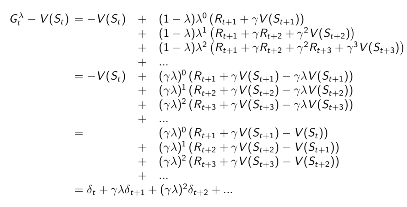
Consider an episode where \(s\) is visited once at time-step \(k\), TD(\(\lambda\)) eligibility trace discounts time since visit, \[ E_t(s) = \gamma\lambda E_{t-1}(s)+1(S_t = s) = \begin{cases} 0, & \mbox{if }t<k \\ (\gamma\lambda)^{t-k}, & \mbox{if }t≥k \end{cases} \] Backward TD(\(\lambda\)) updates accumulate error online \[ \sum^{T-1}_{t=1}\alpha\delta_tE_t(s)=\alpha\sum^{T-1}_{t=k}(\gamma\lambda)^{t-k}\delta_t = \alpha(G_k^\lambda-V(S_k)) \] By end of episode it accumulates total error for \(\lambda\)-return.
For multiple visits to \(s\), \(E_t(s)\) accumulates many errors.
Offline Updates
- Updates are accumulated within episode but applied in batch at the end of episode
Online Updates
- TD(\(\lambda\)) updates are applied online at each step within episode, forward and backward view TD(\(\lambda\)) are slightly different.
In summary,
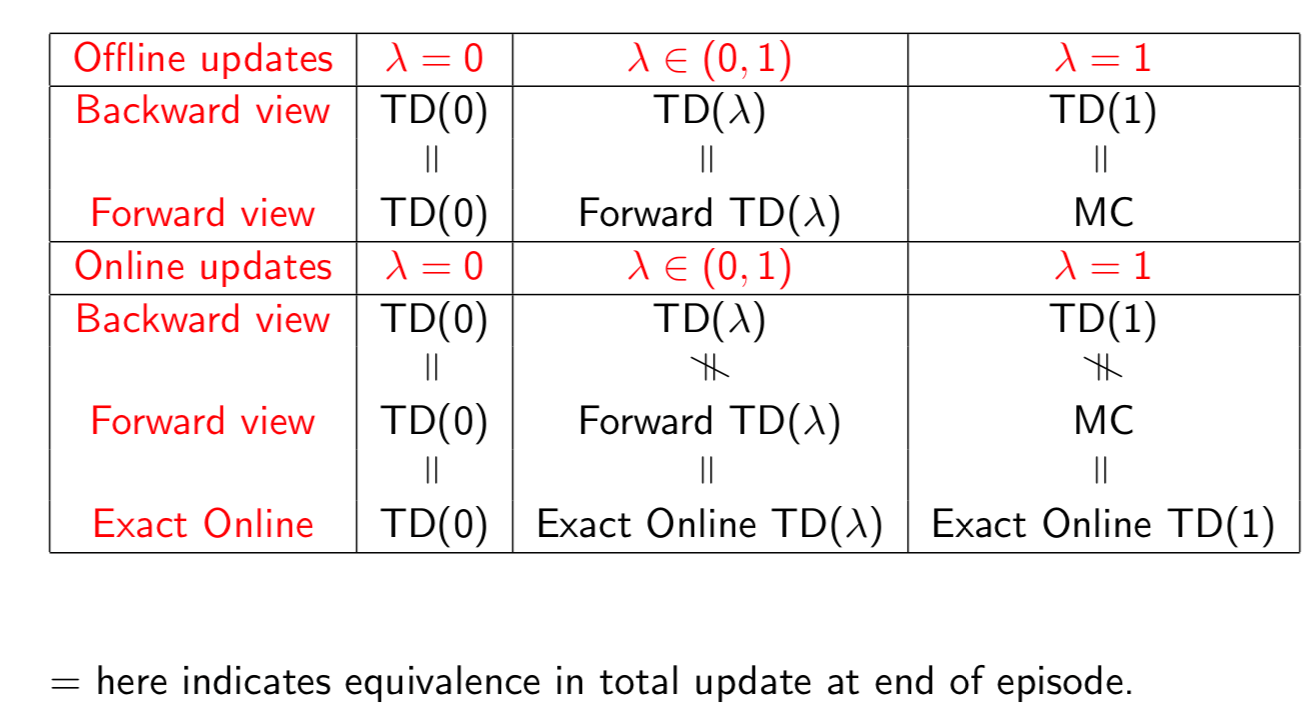
- Forward view provides theory
- Backward view provids mechanism
- update online, every step, from incomplete sequences
This lecture just talks about how to evaluate a policy given an unknown MDP. Next lecture will introduce Model-free Control.