Table of Contents
- Introduction
- Policy Evaluation
- Policy Iteration
- Value Iteration
- Extentions to Dynamic Programming
- Contraction Mapping
Introduction
What is Dynamic Programming?
Dynamic: sequential or temporal component to the problem Programming: optimising a "program", i.e. a policy
- c.f. linear programming
So, Dynamic Programming is a method for solving complex problems by breaking them down into subproblems.
- Solve the subproblems
- Combine solutions to subproblems
Dynamic Programming is a very general solution method for problems which have two properties:
- Optimal substructure
- Principle of optimality applies
- Optimal solution can be decomposed into subproblems
- Overlapping subproblems
- Subproblems recur many times
- Solution can be cached and reused
Markov decision processes satisfy both properties:
- Bellman euqtion gives recursive decomposition
- Value function stores and reuses solutions
Planning by Dynamic Programming
Planning means dynamic programming assumes full knowledge of the MDP.
- For prediction (Policy Evaluation):
- Input: MDP\(<S,A,P,R,\gamma>\) and policy \(\pi\)
- Output: value function \(v_{\pi}\)
- For control:
- Input: MDP\(<S,A,P,R,\gamma>\)
- Output: optimal value function \(v_*\) and optimal policy \(\pi_*\)
We first learn how to evaluate a policy and then put it into a loop to find the optimal policy.
Policy Evaluation
Problem: evaluate a given policy \(\pi\)
Solution: iterative application of Bellman expectation equation
\(v_1\) -> \(v_2\) -> \(v_3\) -> … -> \(v_\pi\)
Synchronous backups
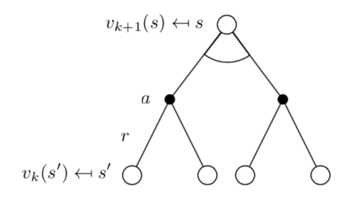
At each iteration \(k+1\)
For all states \(s \in S\)
Update \(v_{k+1}(s)\) from \(v_k(s')\), where \(s'\) is a successor state of \(s\)
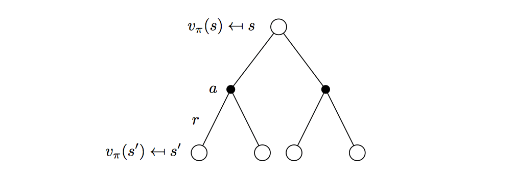 \[
v_{k+1}(s)=\sum_{a\in\mathcal{A}}\pi(a|s)(\mathcal{R}^a_s+\gamma\sum_{s'\in\mathcal{S}}P^a_{ss'}v_k(s'))
\]
\[
v_{k+1}(s)=\sum_{a\in\mathcal{A}}\pi(a|s)(\mathcal{R}^a_s+\gamma\sum_{s'\in\mathcal{S}}P^a_{ss'}v_k(s'))
\]\[ v^{k+1}=\mathcal{R}^\pi+\gamma \mathcal{P}^\pi v^k \]
Example: Evaluating a Random Policy in the Small Gridworld
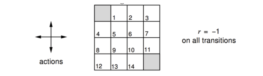
Actions are move North/East/South/West for one grid.
Undiscounted episodic MDP (\(\gamma = 1\))
Nontermial states \(1, …, 14\)
One terminal State (shown twice as shaded squares)
Reward is \(-1\) until the terminal state is reahed
Agent follows uniform random policy \[ \pi(n|\cdot)=\pi(e|\cdot)=\pi(s|\cdot)=\pi(w|\cdot) = 0.25 \]
Let's use dynamic programming to solve the MDP.
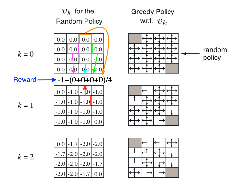
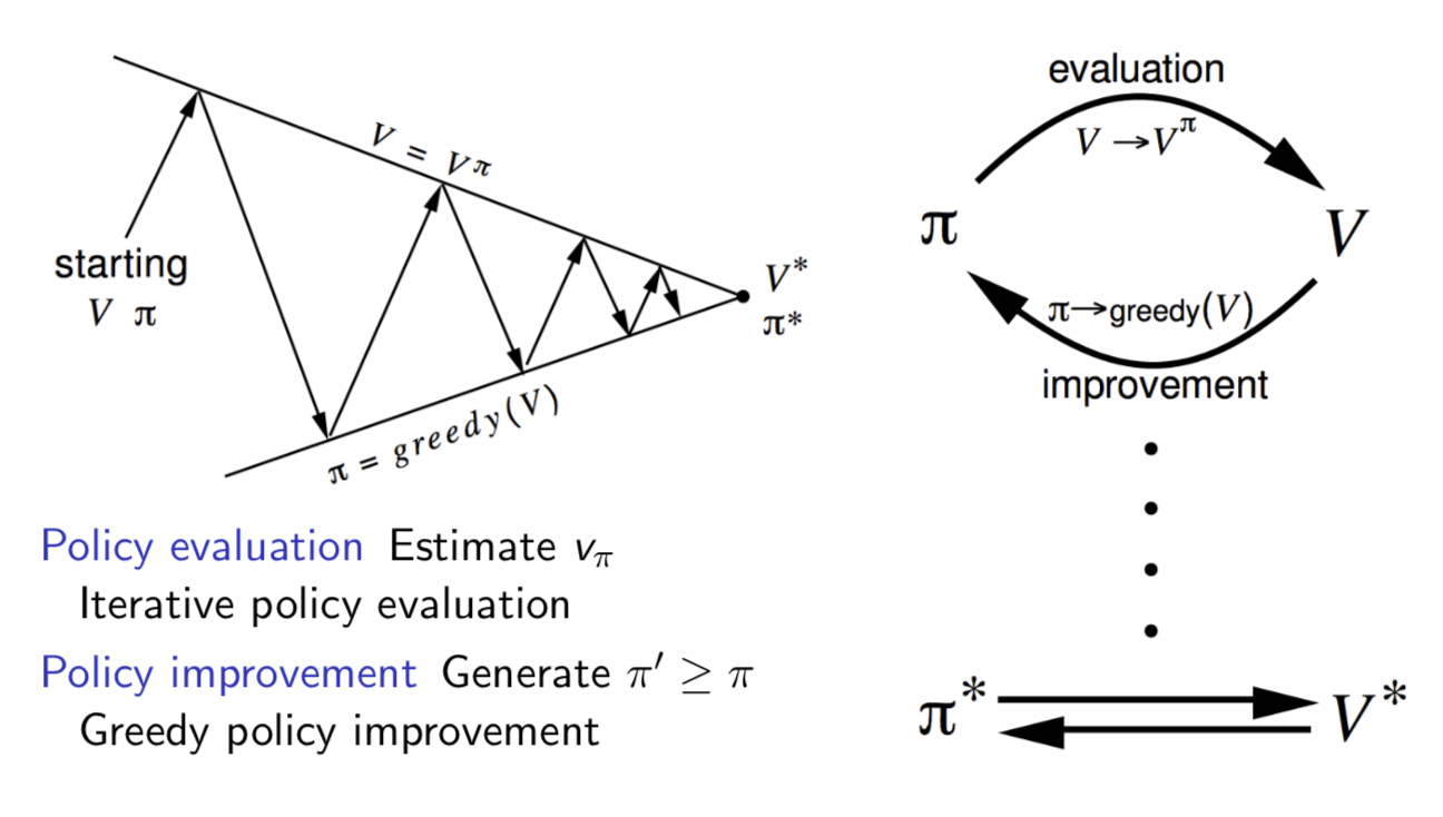
The grids on the left show the value function of each state, the update rule shown by the illustration. Finally, it converges to the true value function of the policy. It basically tell us if we take the random walk under the policy, how much reward on average we will get when we reach the terminal state.
The right-hand column shows how to find better policy with respect to the value funtions.
Policy Iteration
How to improve a Policy
Given a policy \(\pi\)
Evaluate the policy \(\pi\) \[ v_\pi(s) = E[R_{t+1}+\gamma R_{t+2} + ... | S_t = s] \]
Improve the policy by acting greedily with respect to \(v_\pi\) \[ \pi'=greddy(v_\pi) \]
In general, need more iterations of improvement / evaluation
But this process of policy iteration always converges to \(\pi_*\)
Demonstration
Consider a deterministic policy \(a = \pi(s)\), we can improve the policy by acting greedily \[ \pi'(s) = \arg\max_{a\in\mathcal{A}}q_\pi(s, a) \] (Note: \(q_\pi\) is the action value function following policy \(\pi\))
This improves the value from any state \(s\) over one step, \[ q_\pi(s, \pi'(s)) = \max_{a\in\mathcal{A}}q_\pi(s,a)≥q_\pi(s, \pi(s))=v_\pi(s) \] (Note: \(q_\pi(s, \pi'(s))\) means the action value of taking one step following policy \(\pi'\) then following policy \(\pi\) forever.)
If therefore improves the value function, \(v_{\pi'}(s) ≥ v_\pi (s)\) \[ \begin{align} v_\pi(s) & ≤ q_\pi(s, \pi'(s))=E_{\pi'}[R_{t+1}+\gamma v_\pi(S_{t+1})|S_t = s] \\ & ≤ E_{\pi'}[R_{t+1} + \gamma q_\pi(S_{t+1}, \pi'(S_{t+1}))|S_t=s] \\ &≤ E_{\pi'}[R_{t+1} + \gamma R_{t+2} + \gamma^2q_\pi(S_{t+2}, \pi'(S_{t+2}))|S_t = s]\\ &≤ E_{\pi'}[R_{t+1} + \gamma R_{t+2} + ..... | S_t = s] = v_{\pi'}(s) \end{align} \] (Unroll the equation to the second, third … step by taking the Bellman euqation into it.)
If improvements stop, \[ q_\pi(s, \pi'(s)) = \max_{a\in\mathcal{A}}q_\pi(s,a) = q_\pi(s, \pi(s)) = v_\pi(s) \] Then the Bellman optimality equation has been satisfied \[ v_\pi(s) = \max_{a\in\mathcal{A}}q_\pi(s, a) \] Therefore \(v_\pi(s) = v_*(s)\) for all \(s \in \mathcal{S}\), so \(\pi\) is an optimal policy.
Early Stopping
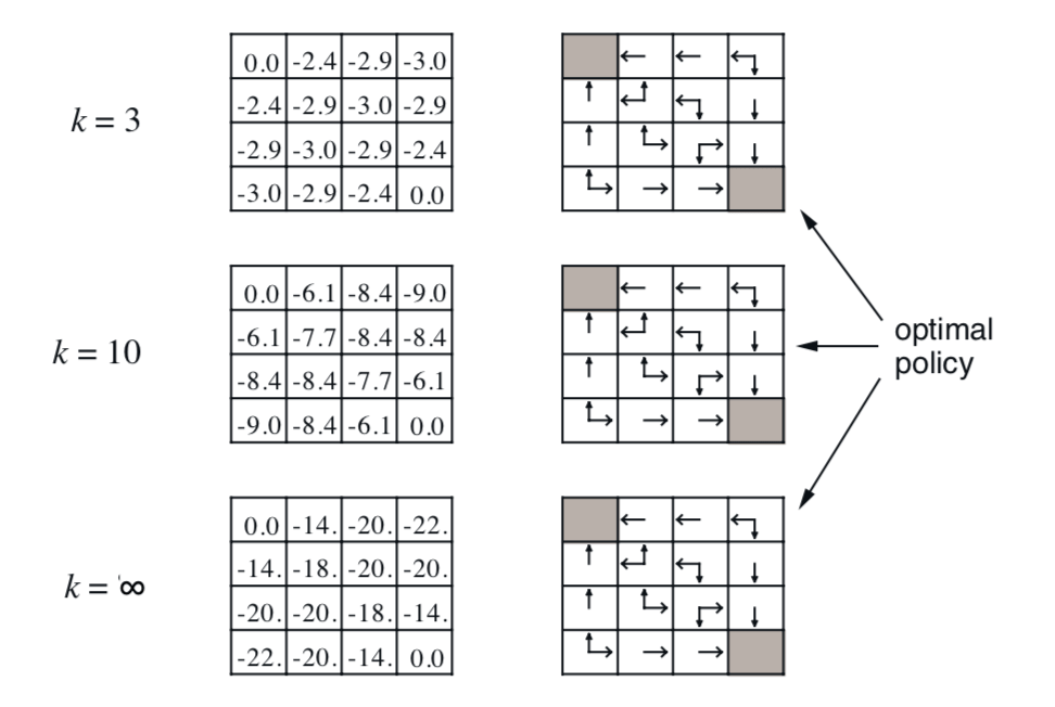
Question: Does policy evaluation need to converge to \(v_\pi\) ?
- e.g. in the small gridworld \(k = 3\) was sufficient to acheive optimal policy
Or shoule we introduce a stopping condition
- e.g. \(\epsilon\)-convergence of value function
Or simply stop after \(k\) iterations of iterative policy evaluation?
Value Iteration
Principle of Optimality
Any optimal policy can be subdivided into two components:
- An optimal first action \(A_*\)
- Followed by an optimal policy from successor state \(S'\)
Theorem: Principle of Optimality
A policy \(\pi(a|s)\) achieves the optimal value from state \(s\), \(v_\pi(s) = v_*(s)\) if and only if
- For any state \(s'\) reachable from \(s\), \(\pi\) achieves the optimal value from state \(s'\)
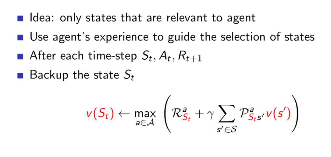
If we know the solution to subproblems \(v_\ast(s')\), then solution \(v_\ast(s)\) can be found by one-step look ahead: \[ v_\ast(s) \leftarrow \max_{a\in\mathcal{A}}\mathcal{R}^a_s+\gamma \sum_{s'\in \mathcal{S}}P^a_{ss'}v_\ast(s') \] The idea of value iteration is to apply these updates iteratively.
- Intuition: start with final rewards and work backwards
- Still works with loopy, stochatis MDPs
Example: Shortest Path
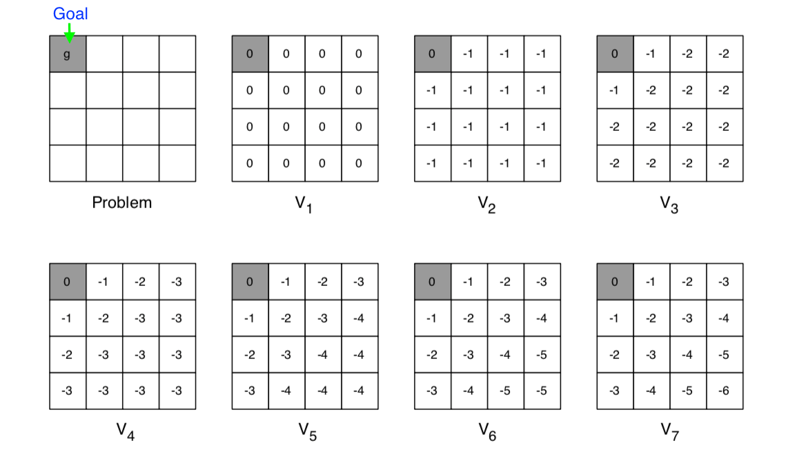
- The goal state is on the left-up corner
- Each step get -1 reward
- The number showed in each grid is the value of that state
- At each iteration, update all states
Value Iteration
- Problem: find optimal policy \(\pi\)
- Solution: iterative application of Bellman optimality backup
- \(v_1 \rightarrow v_2 \rightarrow … \rightarrow v_*\)
- Synchronous backups
- At each iteration \(k+1\)
- For all states \(s\in \mathcal{S}\)
- Update \(v_{k+1}(s)\) from \(v_k(s')\)
- Convergence to \(v_*\) will be proven later
- Unlike policy iteration, there is no explicit policy
- Intermediate value functions may not correspond to any policy
Synchronous Dynamic Programming Algorithms
| problem | bellman equation | algorithm |
|---|---|---|
| Prediction | Bellman Expectation Equation | Iterative Policy Evaluation |
| Control | Bellman Expectation Equation + Greedy Policy Improvement | Policy Iteration |
| Control | Bellman Optimatility Equation | Value Iteration |
Algorithms are based on state-value function \(v_\pi(s)\) or \(v_*(s)\)
- \(O(mn^2)\) per iteration, for \(m\) actions and \(n\) states
Could also apply to action-value function \(q_\pi(s, a)\) or \(q_*(s, a)\)
- \(O(m^2n^2)\) per iteration
Extentions to Dynamic Programming
Asynchronous Dynamic Programming
Asynchronous DP backs up states individually, in any order. For each selected state, apply the appropriate backup, which can significantly reduce computation. It also guaranteed to converge if all states continue to be selected.
Three simple ideas for asynchronous dynamic programming:
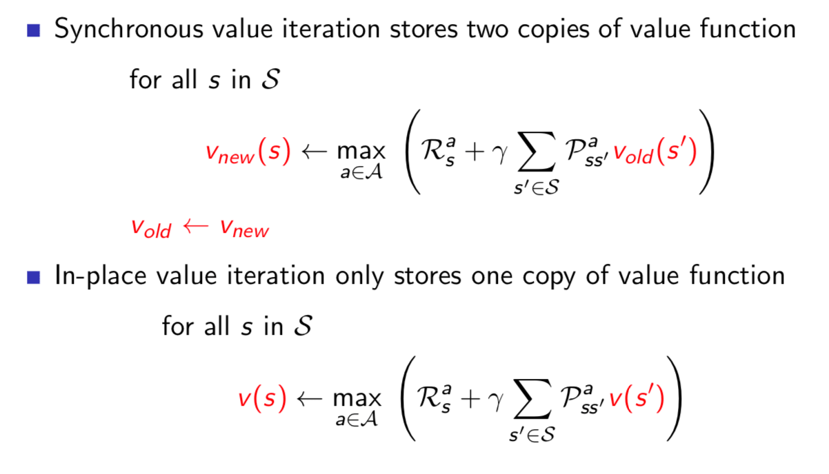
In-place dynamic programming
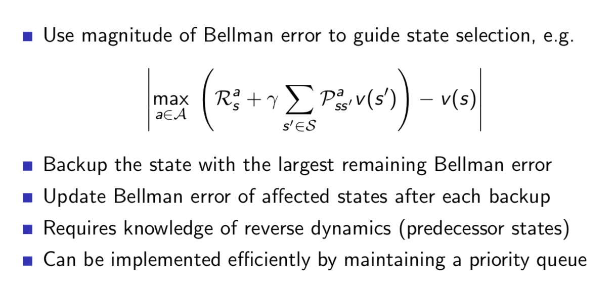
Prioritised sweeping
Real-time dynamic programming
Full-Width Backups
DP uses full-width backups
- full-width means when we look aheah, we consider all branches(actions) that could happen
- For each backup (sync or async)
- Every successor state and action is considered
- Using knowledge of the MDP transitions and reward function
Contraction Mapping
Information about contraction mapping theorem, please refer to http://www.math.uconn.edu/~kconrad/blurbs/analysis/contraction.pdf
Consider the vector space \(\mathcal{V}\) over value functions. There are \(|\mathcal{S}|\) dimensions.
- Each point in this space fully specifies a value function \(v(s)\)
We will measure distance between state-value functions \(u\) and \(v\) by the \(\infty\)-norm. \[ ||u-v||_\infty = \max_{s\in\mathcal{S}}|u(s)-v(s)| \] Bellman Expectation Backup is a Contraction
Define the Bellman expectation backup operator \(T^\pi\), \[ T^\pi(v) = \mathcal{R}^\pi + \gamma\mathcal{P}^\pi v \] This operator is a \(\gamma\)-contraction, it makes value functions closer bt at least \(\gamma\), \[ \begin{align} ||T^\pi(u)-T^\pi(v)||_\infty &= ||(\mathcal{R}^\pi + \gamma\mathcal{P}^\pi v) - (\mathcal{R}^\pi + \gamma\mathcal{P}^\pi u)||_\infty \\ &= ||\gamma P^\pi(u-v)||_\infty\\ &≤||\gamma P^\pi||u-v||_\infty||_\infty\\ &≤\gamma||u-v||_\infty \end{align} \]
Theorem: Contraction Mapping Theorem
For any metric space \(\mathcal{V}\) that is complete (closed) under an operator \(T(v)\), where \(T\) is a \(\gamma\)-contraction,
- \(T\) converges to a unique fixed point
- At a linear convergence rate of \(\gamma\)
Convergence of Iterative Policy Evaluation and Policy Iteration
The Bellman expectation operator \(T^\pi\) has a unique fixed point \(v_\pi\).
By contraction mapping theorem,
- Iterative policy evaluation converges on \(v_\pi\);
- Policy iteration converges on \(v_*\).
Bellman Optimality Backup is a Contraction
Define the Bellman Optimality backup operator \(T^\ast\), \[ T^\ast(v) = \max_{a\in\mathcal{A}}\mathcal{R}^a+\gamma \mathcal{P}^av \] This operator is a \(\gamma\)-contraction, it makes value functions closer by at least \(\gamma\), \[ ||T^\ast(u)-T\ast(v)||_\infty≤\gamma ||u-v||_\infty \] Convergence of Value Iteration
The Bellman optimality operator \(T^∗\) has a unique fixed point \(v_*\).
By contraction mapping theorem, value iteration converges on \(v_*\).
In summary, what does a Bellman backup do to points in value function space is to bring value functions closer to a unique fixed point. And therefore the backups must converge on a unique solution.
This lecture (note) introduces how to use dynamic programming to solve planning problems. Next lecture will introduce model-free prediction, which is a really RL problem.